Kafka Streams Domain Specific Language for Confluent Platform
The Kafka Streams DSL (Domain Specific Language) is built on top of the Streams Processor API. It is recommended for most users, especially beginners. Most data processing operations can be expressed in just a few lines of DSL code.
Overview
In comparison to the Processor API, only the DSL supports:
Built-in abstractions for streams and tables in the form of KStream, KTable, and GlobalKTable. Having first-class support for streams and tables is crucial because, in practice, most use cases require not just either streams or databases/tables, but a combination of both. For example, if your use case is to create a customer 360-degree view that is updated in real-time, what your application will be doing is transforming many input streams of customer-related events into an output table that contains a continuously updated 360-degree view of your customers.
Declarative, functional programming style with stateless transformations (e.g.,
mapandfilter) as well as stateful transformations such as aggregations (e.g.,countandreduce), joins (e.g.,leftJoin), and windowing (e.g., session windows).
With the DSL, you can define processor topologies (that is, the logical processing plan) in your application. The steps to accomplish this are:
Specify one or more input streams that are read from Kafka topics.
Compose transformations on these streams.
Write the resulting output streams back to Kafka topics, or expose the processing results of your application directly to other applications through Kafka Streams Interactive Queries for Confluent Platform (e.g., via a REST API).
After the application is run, the defined processor topologies are continuously executed (that is, the processing plan is put into action). A step-by-step guide for writing a stream processing application using the DSL is provided below.
Once you have built your Kafka Streams application using the DSL you can view the underlying Topology by first executing StreamsBuilder#build() which returns the Topology object. Then to view the Topology you call Topology#desribe(). Full details on describing a Topology can be found in describing a topology.
For a complete list of available API functionality, see also the Kafka Streams Javadocs.
Creating source streams from Kafka
You can easily read data from Apache Kafka® topics into your application. The following operations are supported.
Reading from Kafka | Description |
|---|---|
Stream
| Creates a KStream from the specified Kafka input topics and interprets the data as a record stream. A In the case of a KStream, the local KStream instance of every application instance will be populated with data from only a subset of the partitions of the input topic. Collectively, across all application instances, all input topic partitions are read and processed. import org.apache.kafka.common.serialization.Serdes;
import org.apache.kafka.streams.StreamsBuilder;
import org.apache.kafka.streams.kstream.KStream;
StreamsBuilder builder = new StreamsBuilder();
KStream<String, Long> wordCounts = builder.stream(
"word-counts-input-topic", /* input topic */
Consumed.with(
Serdes.String(), /* key serde */
Serdes.Long() /* value serde */
);
If you do not specify Serdes explicitly, the default Serdes from the configuration are used. You must specify Serdes explicitly if the key or value types of the records in the Kafka input topics do not match the configured default Serdes. For information about configuring default Serdes, available Serdes, and implementing your own custom Serdes see Kafka Streams Data Types and Serialization for Confluent Platform. Several variants of Kafka Streams assumes that input topics are already partitioned by key, which means that |
Table
| Reads the specified Kafka input topic into a KTable. The topic is interpreted as a changelog stream, where records with the same key are interpreted as UPSERT aka INSERT/UPDATE (when the record value is not In the case of a KTable, the local KTable instance of every application instance will be populated with data from only a subset of the partitions of the input topic. Collectively, across all application instances, all input topic partitions are read and processed. You must provide a name for the table (more precisely, for the internal state store that backs the table). This is required for supporting Kafka Streams Interactive Queries for Confluent Platform against the table. When a name is not provided, the table is not queryable, and an internal name is provided for the state store. If you do not specify Serdes explicitly, the default Serdes from the configuration are used. You must specify Serdes explicitly if the key or value types of the records in the Kafka input topics do not match the configured default Serdes. For information about configuring default Serdes, available Serdes, and implementing your own custom Serdes see Kafka Streams Data Types and Serialization for Confluent Platform. Several variants of |
Global Table
| Reads the specified Kafka input topic into a GlobalKTable. The topic is interpreted as a changelog stream, where records with the same key are interpreted as UPSERT aka INSERT/UPDATE (when the record value is not In the case of a GlobalKTable, the local GlobalKTable instance of every application instance will be populated with data from all input topic partitions. Collectively, across all application instances, all input topic partitions are consumed by all instances of the application. You must provide a name for the table (more precisely, for the internal state store that backs the table). This is required for supporting Kafka Streams Interactive Queries for Confluent Platform against the table. When a name is not provided, the table is not queryable, and an internal name is provided for the state store. import org.apache.kafka.common.serialization.Serdes;
import org.apache.kafka.streams.StreamsBuilder;
import org.apache.kafka.streams.kstream.GlobalKTable;
StreamsBuilder builder = new StreamsBuilder();
GlobalKTable<String, Long> wordCounts = builder.globalTable(
"word-counts-input-topic",
Materialized.<String, Long, KeyValueStore<Bytes, byte[]>>as(
"word-counts-global-store" /* table/store name */)
.withKeySerde(Serdes.String()) /* key serde */
.withValueSerde(Serdes.Long()) /* value serde */
);
You must specify Serdes explicitly if the key or value types of the records in the Kafka input topics do not match the configured default Serdes. For information about configuring default Serdes, available Serdes, and implementing your own custom Serdes see Kafka Streams Data Types and Serialization for Confluent Platform. Several variants of |
Transform a stream
The KStream and KTable interfaces support a variety of transformation operations. Each of these operations can be translated into one or more connected processors into the underlying processor topology. Since KStream and KTable are strongly typed, all of these transformation operations are defined as generic functions where users could specify the input and output data types.
Some KStream transformations may generate one or more KStream objects, for example: - filter and map on a KStream will generate another KStream - split on a KStream can generate multiple KStreams
Some others may generate a KTable object, for example an aggregation of a KStream also yields a KTable. This allows Kafka Streams to continuously update the computed value upon arrivals of out-of-order records after it has already been produced to the downstream transformation operators.
All KTable transformation operations can only generate another KTable. However, the Kafka Streams DSL does provide a special function that converts a KTable representation into a KStream. All of these transformation methods can be chained together to compose a complex processor topology.
These transformation operations are described in the following subsections:
Stateless transformations
Stateless transformations do not require state for processing and they do not require a state store associated with the stream processor. Kafka 0.11.0 and later allows you to materialize the result from a stateless KTable transformation. This allows the result to be queried through Kafka Streams Interactive Queries for Confluent Platform. To materialize a KTable, each of the below stateless operations can be augmented with an optional queryableStoreName argument.
Transformation | Description |
|---|---|
Branch
| Branch (or split) a Predicates are evaluated in order. A record is placed to one and only one output stream on the first match: if the n-th predicate evaluates to true, the record is placed to n-th stream. If no predicate matches, the the record is dropped. Branching is useful, for example, to route records to different downstream topics. KStream<String, Long> stream = ...;
Map<String, KStream<String, Long>> branches =
stream.split(Named.as("Branch-"))
.branch((key, value) -> key.startsWith("A"), /* first predicate */
Branched.as("A"))
.branch((key, value) -> key.startsWith("B"), /* second predicate */
Branched.as("B"))
.defaultBranch(Branched.as("C"))
);
// KStream branches.get("Branch-A") contains all records whose keys start with "A"
// KStream branches.get("Branch-B") contains all records whose keys start with "B"
// KStream branches.get("Branch-C") contains all other records
|
Broadcast/Multicast
| Broadcast a A record is sent to more than one operator by applying multiple operators to the same KStream<String, Long> stream = ...;
KStream<...> stream1 = stream.map(...);
KStream<...> stream2 = stream.mapValue(...);
KStream<...> stream3 = stream.flatMap(...);
Multicast a In contrast to branching, which sends each record to at most one downstream branch, a multicast may send a record to any number of downstream A multicast is implemented as a broadcast plus filters. KStream<String, Long> stream = ...;
// contains all records whose keys start with "A"
KStream<...> stream1 = stream.filter((key, value) -> key.startsWith("A"));
// contains all records whose keys start with "AB" (subset of stream1)
KStream<...> stream2 = stream.filter((key, value) -> key.startsWith("AB"));
// contains all records whose keys contains a "B" (superset of stream2)
KStream<...> stream3 = stream.filter((key, value) -> key.contains("B"));
|
Filter
| Evaluates a boolean function for each element and retains those for which the function returns true. (KStream details, KTable details) KStream<String, Long> stream = ...;
// A filter that selects (keeps) only positive numbers
// Java 8+ example, using lambda expressions
KStream<String, Long> onlyPositives = stream.filter((key, value) -> value > 0);
|
Inverse Filter
| Evaluates a boolean function for each element and drops those for which the function returns true. (KStream details, KTable details) KStream<String, Long> stream = ...;
// An inverse filter that discards any negative numbers or zero
// Java 8+ example, using lambda expressions
KStream<String, Long> onlyPositives = stream.filterNot((key, value) -> value <= 0);
|
FlatMap
| Takes one record and produces zero, one, or more records. You can modify the record keys and values, including their types. (details) Marks the stream for data re-partitioning: Applying a grouping or a join after KStream<Long, String> stream = ...;
KStream<String, Integer> transformed = stream.flatMap(
// Here, we generate two output records for each input record.
// We also change the key and value types.
// Example: (345L, "Hello") -> ("HELLO", 1000), ("hello", 9000)
(key, value) -> {
List<KeyValue<String, Integer>> result = new LinkedList<>();
result.add(KeyValue.pair(value.toUpperCase(), 1000));
result.add(KeyValue.pair(value.toLowerCase(), 9000));
return result;
}
);
|
FlatMap (values only)
| Takes one record and produces zero, one, or more records, while retaining the key of the original record. You can modify the record values and the value type. (details)
// Split a sentence into words.
KStream<byte[], String> sentences = ...;
KStream<byte[], String> words = sentences.flatMapValues(value -> Arrays.asList(value.split("\\s+")));
|
Foreach
| Terminal operation. Performs a stateless action on each record. (details) You would use Note on processing guarantees: Any side effects of an action (such as writing to external systems) are not trackable by Kafka, which means they will typically not benefit from Kafka’s processing guarantees. KStream<String, Long> stream = ...;
// Print the contents of the KStream to the local console.
// Java 8+ example, using lambda expressions
stream.foreach((key, value) -> System.out.println(key + " => " + value));
|
GroupByKey
| Groups the records by the existing key. (details) Grouping is a prerequisite for aggregating a stream or a table and ensures that data is properly partitioned (“keyed”) for subsequent operations. When to set explicit Serdes: Variants of Grouping vs. Windowing: A related operation is windowing, which lets you control how to “sub-group” the grouped records of the same key into so-called windows for stateful operations such as windowed aggregations or windowed joins. Causes data re-partitioning if and only if the stream was marked for re-partitioning. KStream<byte[], String> stream = ...;
// Group by the existing key, using the application's configured
// default serdes for keys and values.
KGroupedStream<byte[], String> groupedStream = stream.groupByKey();
// When the key and/or value types do not match the configured
// default serdes, we must explicitly specify serdes.
KGroupedStream<byte[], String> groupedStream = stream.groupByKey(
Grouped.with(
Serdes.ByteArray(), /* key */
Serdes.String()) /* value */
);
|
GroupBy
| Groups the records by a new key, which may be of a different key type. When grouping a table, you may also specify a new value and value type. Grouping is a prerequisite for aggregating a stream or a table and ensures that data is properly partitioned (“keyed”) for subsequent operations. When to set explicit Serdes: Variants of Grouping vs. Windowing: A related operation is windowing, which lets you control how to “sub-group” the grouped records of the same key into so-called windows for stateful operations such as windowed aggregations or windowed joins. Always causes data re-partitioning: KStream<byte[], String> stream = ...;
KTable<byte[], String> table = ...;
// Java 8+ examples, using lambda expressions
// Group the stream by a new key and key type
KGroupedStream<String, String> groupedStream = stream.groupBy(
(key, value) -> value,
Grouped.with(
Serdes.String(), /* key (note: type was modified) */
Serdes.String()) /* value */
);
// Group the table by a new key and key type, and also modify the value and value type.
KGroupedTable<String, Integer> groupedTable = table.groupBy(
(key, value) -> KeyValue.pair(value, value.length()),
Grouped.with(
Serdes.String(), /* key (note: type was modified) */
Serdes.Integer()) /* value (note: type was modified) */
);
|
Cogroup
| Cogrouping enables aggregating multiple input streams in a single operation. The different (already grouped) input streams must have the same key type and may have different values types. Because each Cogroup does not cause a repartition as it has the prerequisite that the input streams are grouped. In the process of creating these groups they will have already been repartitioned if the stream was already marked for repartitioning. KGroupedStream<byte[], String> groupedStreamOne = ...;
KGroupedStream<byte[], Long> groupedStreamTwo = ...;
// Java 8+ examples, using lambda expressions
// Create new cogroup from the first stream (the value type of the CogroupedStream is the value type of the final aggregation result)
CogroupedStream<byte[], Integer> cogroupedStream = groupedStreamOne.cogroup(
(aggKey, newValue, aggValue) -> aggValue + Integer.parseInteger(newValue) /* adder for first stream */
);
// Add the second stream to the existing cogroup (note, that the second input stream has a different value type than the first input stream)
cogroupedStream.cogroup(
groupedStreamTwo,
(aggKey, newValue, aggValue) -> aggValue + newValue.intValue() /* adder for second stream */
);
// Aggregate all streams of the cogroup
KTable<byte[], Integer> aggregatdTable = cogroup.aggregate(
() -> 0, /* initializer */
Materialized.as("aggregated-stream-store") /* state store name */
.withValueSerde(Serdes.Integer() /* serde for aggregate value */
);
|
Map
| Takes one record and produces one record. You can modify the record key and value, including their types. (details) Marks the stream for data re-partitioning: Applying a grouping or a join after KStream<byte[], String> stream = ...;
// Java 8+ example, using lambda expressions
// Note how we change the key and the key type (similar to `selectKey`)
// as well as the value and the value type.
KStream<String, Integer> transformed = stream.map(
(key, value) -> KeyValue.pair(value.toLowerCase(), value.length()));
|
Map (values only)
| Takes one record and produces one record, while retaining the key of the original record. You can modify the record value and the value type. (KStream details, KTable details)
KStream<byte[], String> stream = ...;

// Java 8+ example, using lambda expressions
KStream<byte[], String> uppercased = stream.mapValues(value -> value.toUpperCase());
|
Merge
| Merges records of two streams into one larger stream. (details) There is no ordering guarantee between records from different streams in the merged stream. Relative order is preserved within each input stream though (ie, records within the same input stream are processed in order). KStream<byte[], String> stream1 = ...;
KStream<byte[], String> stream2 = ...;
KStream<byte[], String> merged = stream1.merge(stream2);
|
Peek
| Performs a stateless action on each record, and returns an unchanged stream. (details) You would use
Note on processing guarantees: Any side effects of an action (such as writing to external systems) are not trackable by Kafka, which means they will typically not benefit from Kafka’s processing guarantees. KStream<byte[], String> stream = ...;
// Java 8+ example, using lambda expressions
KStream<byte[], String> unmodifiedStream = stream.peek(
(key, value) -> System.out.println("key=" + key + ", value=" + value));
|
| Terminal operation. Prints the records to Calling KStream<byte[], String> stream = ...;
// print to sysout
stream.print(Printed.toSysOut());
// print to file with a custom label
stream.print(Printed.toFile("streams.out").withLabel("streams"));
|
Repartition
| Manually trigger repartitioning of the stream with the specified number of partitions. (details) Kafka Streams manages the topic for KStream<byte[], String> stream = ... ;
KStream<byte[], String> repartitionedStream = stream.repartition(Repartitioned.numberOfPartitions(10));
|
SelectKey
| Assigns a new key – possibly of a new key type – to each record. (details) Calling Marks the stream for data re-partitioning: Applying a grouping or a join after KStream<byte[], String> stream = ...;
// Derive a new record key from the record's value. Note how the key type changes, too.
// Java 8+ example, using lambda expressions
KStream<String, String> rekeyed = stream.selectKey((key, value) -> value.split(" ")[0])
|
Stream to Table
| Convert an event stream into a table or a changelog stream. (details) KStream<byte[], String> stream = ...;
KTable<byte[], String> table = stream.toTable();
|
Table to Stream
| Get the changelog stream of this table. (details) KTable<byte[], String> table = ...;
// Also, a variant of `toStream` exists that allows you
// to select a new key for the resulting stream.
KStream<byte[], String> stream = table.toStream();
|
Stateful transformations
Stateful transformations depend on state for processing inputs and producing outputs and require a state store associated with the stream processor. For example, in aggregating operations, a windowing state store is used to collect the latest aggregation results per window. In join operations, a windowing state store is used to collect all of the records received so far within the defined window boundary.
State stores are fault-tolerant. In case of failure, Kafka Streams guarantees to fully restore all state stores prior to resuming the processing. For more information, see Fault tolerance.
Available stateful transformations in the DSL include:
Windowing (as part of aggregations and joins)
Applying custom processors and transformers, which may be stateful, for Processor API integration
The following diagram shows their relationships:
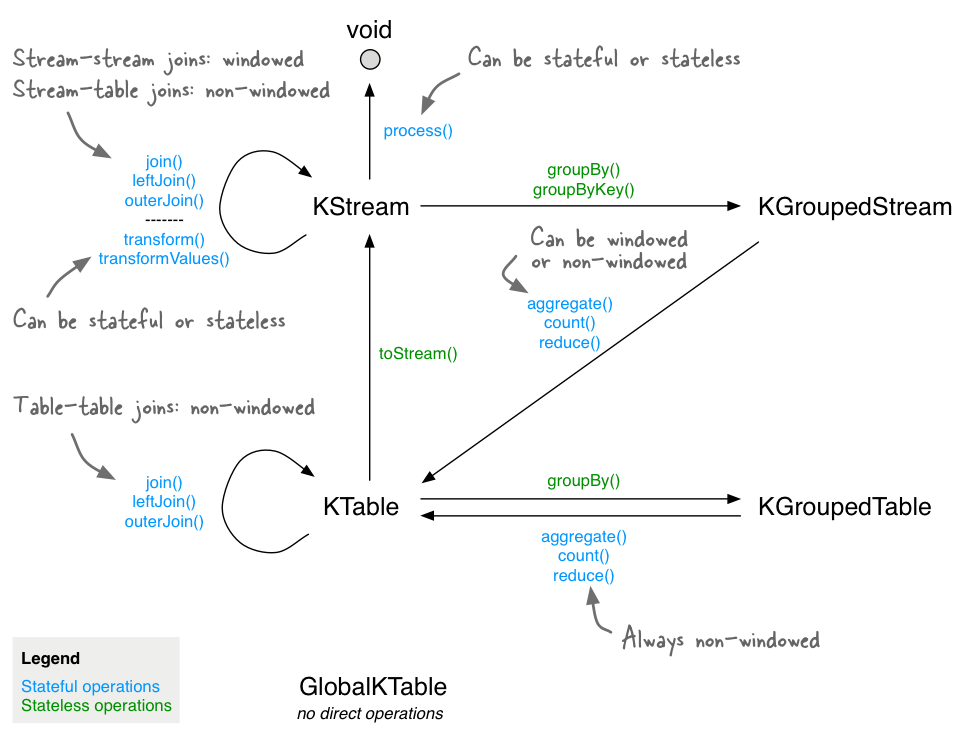
Stateful transformations in the DSL.
Here is an example of a stateful application: the WordCount algorithm.
WordCount example in Java 8+, using lambda expressions (see here for the full code):
// Assume the record values represent lines of text.  For the sake of this example, you can ignore
// whatever may be stored in the record keys.
KStream<String, String> textLines = ...;

KStream<String, Long> wordCounts = textLines
    // Split each text line, by whitespace, into words.  The text lines are the record
    // values, that is, you can ignore whatever data is in the record keys and thus invoke
    // `flatMapValues` instead of the more generic `flatMap`.
    .flatMapValues(value -> Arrays.asList(value.toLowerCase().split("\\W+")))
    // Group the stream by word to ensure the key of the record is the word.
    .groupBy((key, word) -> word)
    // Count the occurrences of each word (record key).
    //
    // This will change the stream type from `KGroupedStream<String, String>` to
    // `KTable<String, Long>` (word -> count).
    .count()
    // Convert the `KTable<String, Long>` into a `KStream<String, Long>`.
    .toStream();
Aggregating
After records are grouped by key via groupByKey or groupBy – and thus represented as either a KGroupedStream or a KGroupedTable, they can be aggregated via an operation such as reduce. Aggregations are key-based operations, which means that they always operate over records (notably record values) of the same key. You can perform aggregations on windowed or non-windowed data.
Important
To support fault tolerance and avoid undesirable behavior, the initializer and aggregator must be stateless. The aggregation results should be passed in the return value of the initializer and aggregator. Do not use class member variables because that data can potentially get lost in case of failure.
Transformation | Description |
|---|---|
Aggregate
| Rolling aggregation. Aggregates the values of (non-windowed) records by the grouped key. Aggregating is a generalization of When aggregating a grouped stream, you must provide an initializer (e.g., Several variants of KGroupedStream<byte[], String> groupedStream = ...;
KGroupedTable<byte[], String> groupedTable = ...;
// Java 8+ examples, using lambda expressions
// Aggregating a KGroupedStream (note how the value type changes from String to Long)
KTable<byte[], Long> aggregatedStream = groupedStream.aggregate(
() -> 0L, /* initializer */
(aggKey, newValue, aggValue) -> aggValue + newValue.length(), /* adder */
Materialized.as("aggregated-stream-store") /* state store name */
.withValueSerde(Serdes.Long()) /* serde for aggregate value */
);
// Aggregating a KGroupedTable (note how the value type changes from String to Long)
KTable<byte[], Long> aggregatedTable = groupedTable.aggregate(
() -> 0L, /* initializer */
(aggKey, newValue, aggValue) -> aggValue + newValue.length(), /* adder */
(aggKey, oldValue, aggValue) -> aggValue - oldValue.length(), /* subtractor */
Materialized.as("aggregated-table-store") /* state store name */
.withValueSerde(Serdes.Long()) /* serde for aggregate value */
);
Detailed behavior of
Detailed behavior of
See the example at the bottom of this section for a visualization of the aggregation semantics. |
Aggregate (windowed)
| Windowed aggregation. Aggregates the values of records, per window, by the grouped key. Aggregating is a generalization of When aggregating a grouped stream, you must provide an initializer (e.g., The windowed Several variants of import java.time.Duration;
KGroupedStream<String, Long> groupedStream = ...;
CogroupedKStream<String, Long> cogroupedStream = ...;
// Java 8+ examples, using lambda expressions
// Aggregating with time-based windowing (here: with 5-minute tumbling windows)
KTable<Windowed<String>, Long> timeWindowedAggregatedStream = groupedStream.windowedBy(TimeWindows.of(Duration.ofMinutes(5)))
.aggregate(
() -> 0L, /* initializer */
(aggKey, newValue, aggValue) -> aggValue + newValue, /* adder */
Materialized.<String, Long, WindowStore<Bytes, byte[]>>as("time-windowed-aggregated-stream-store") /* state store name */
.withValueSerde(Serdes.Long())); /* serde for aggregate value */
// Aggregating with time-based windowing (here: with 5-minute tumbling windows)
// (note: the required "adder" aggregator is specified in the prior `cogroup()` call already)
KTable<Windowed<String>, Long> timeWindowedAggregatedStream = cogroupedStream.windowedBy(TimeWindows.of(Duration.ofMinutes(5)))
.aggregate(
() -> 0L, /* initializer */
Materialized.<String, Long, WindowStore<Bytes, byte[]>>as("time-windowed-aggregated-stream-store") /* state store name */
.withValueSerde(Serdes.Long())); /* serde for aggregate value */
// Aggregating with time-based windowing (here: with 5-minute sliding windows and 30-minute grace period)
KTable<Windowed<String>, Long> timeWindowedAggregatedStream = groupedStream
.windowedBy(SlidingWindows.withTimeDifferenceAndGrace(Duration.ofMinutes(5), Duration.ofMinutes(30)))
.aggregate(
() -> 0L, /* initializer */
(aggKey, newValue, aggValue) -> aggValue + newValue, /* adder */
Materialized.<String, Long, WindowStore<Bytes, byte[]>>as("time-windowed-aggregated-stream-store") /* state store name */
.withValueSerde(Serdes.Long())); /* serde for aggregate value */
// Aggregating with time-based windowing (here: with 5-minute sliding windows and 30-minute grace period)
// (note: the required "adder" aggregator is specified in the prior `cogroup()` call already)
KTable<Windowed<String>, Long> timeWindowedAggregatedStream = cogroupedStream
.windowedBy(SlidingWindows.withTimeDifferenceAndGrace(Duration.ofMinutes(5), Duration.ofMinutes(30)))
.aggregate(
() -> 0L, /* initializer */
Materialized.<String, Long, WindowStore<Bytes, byte[]>>as("time-windowed-aggregated-stream-store") /* state store name */
.withValueSerde(Serdes.Long())); /* serde for aggregate value */
// Aggregating with session-based windowing (here: with an inactivity gap of 5 minutes)
KTable<Windowed<String>, Long> sessionizedAggregatedStream = groupedStream.windowedBy(SessionWindows.with(Duration.ofMinutes(5)).
aggregate(
() -> 0L, /* initializer */
(aggKey, newValue, aggValue) -> aggValue + newValue, /* adder */
(aggKey, leftAggValue, rightAggValue) -> leftAggValue + rightAggValue, /* session merger */
Materialized.<String, Long, SessionStore<Bytes, byte[]>>as("sessionized-aggregated-stream-store") /* state store name */
.withValueSerde(Serdes.Long())); /* serde for aggregate value */
// Aggregating with session-based windowing (here: with an inactivity gap of 5 minutes)
// (note: the required "adder" aggregator is specified in the prior `cogroup()` call already)
KTable<Windowed<String>, Long> sessionizedAggregatedStream = cogroupedStream.windowedBy(SessionWindows.with(Duration.ofMinutes(5)).
aggregate(
() -> 0L, /* initializer */
(aggKey, leftAggValue, rightAggValue) -> leftAggValue + rightAggValue, /* session merger */
Materialized.<String, Long, SessionStore<Bytes, byte[]>>as("sessionized-aggregated-stream-store") /* state store name */
.withValueSerde(Serdes.Long())); /* serde for aggregate value */
Detailed behavior:
See the example at the bottom of this section for a visualization of the aggregation semantics. |
Count
| Rolling aggregation. Counts the number of records by the grouped key. (KGroupedStream details, KGroupedTable details) Several variants of KGroupedStream<String, Long> groupedStream = ...;
KGroupedTable<String, Long> groupedTable = ...;
// Counting a KGroupedStream
KTable<String, Long> aggregatedStream = groupedStream.count();
// Counting a KGroupedTable
KTable<String, Long> aggregatedTable = groupedTable.count();
Detailed behavior for
Detailed behavior for
|
Count (windowed)
| Windowed aggregation. Counts the number of records, per window, by the grouped key. (TimeWindowedKStream details, SessionWindowedKStream details) The windowed Several variants of import java.time.Duration;
KGroupedStream<String, Long> groupedStream = ...;
// Counting a KGroupedStream with time-based windowing (here: with 5-minute tumbling windows)
KTable<Windowed<String>, Long> aggregatedStream = groupedStream.windowedBy(
TimeWindows.of(Duration.ofMinutes(5))) /* time-based window */
.count();
// Counting a KGroupedStream with sliding windows time-based windowing (here: with 5-minute sliding windows and 30-minute grace period)
KTable<Windowed<String>, Long> aggregatedStream = groupedStream.windowedBy(
SlidingWindows.withTimeDifferenceAndGrace(Duration.ofMinutes(5), Duration.ofMinutes(30))) /* time-based window */
.count();
// Counting a KGroupedStream with session-based windowing (here: with 5-minute inactivity gaps)
KTable<Windowed<String>, Long> aggregatedStream = groupedStream.windowedBy(
SessionWindows.with(Duration.ofMinutes(5))) /* session window */
.count();
Detailed behavior:
|
Reduce
| Rolling aggregation. Combines the values of (non-windowed) records by the grouped key. The current record value is combined with the last reduced value, and a new reduced value is returned. The result value type cannot be changed, unlike When reducing a grouped stream, you must provide an “adder” reducer (e.g., Several variants of KGroupedStream<String, Long> groupedStream = ...;
KGroupedTable<String, Long> groupedTable = ...;
// Java 8+ examples, using lambda expressions
// Reducing a KGroupedStream
KTable<String, Long> aggregatedStream = groupedStream.reduce(
(aggValue, newValue) -> aggValue + newValue /* adder */);
// Reducing a KGroupedTable
KTable<String, Long> aggregatedTable = groupedTable.reduce(
(aggValue, newValue) -> aggValue + newValue, /* adder */
(aggValue, oldValue) -> aggValue - oldValue /* subtractor */);
Detailed behavior for
Detailed behavior for
See the example at the bottom of this section for a visualization of the aggregation semantics. |
Reduce (windowed)
| Windowed aggregation. Combines the values of records, per window, by the grouped key. The current record value is combined with the last reduced value, and a new reduced value is returned. Records with The windowed Several variants of import java.time.Duration;
KGroupedStream<String, Long> groupedStream = ...;
// Java 8+ examples, using lambda expressions
// Aggregating with time-based windowing (here: with 5-minute tumbling windows)
KTable<Windowed<String>, Long> timeWindowedAggregatedStream = groupedStream.windowedBy(
TimeWindows.of(Duration.ofMinutes(5)) /* time-based window */)
.reduce(
(aggValue, newValue) -> aggValue + newValue /* adder */
);
// Aggregating with time-based windowing (here: with 5-minute sliding windows and 30-minute grace period)
KTable<Windowed<String>, Long> timeWindowedAggregatedStream = groupedStream
.windowedBy(SlidingWindows.withTimeDifferenceAndGrace(Duration.ofMinutes(5), Duration.ofMinutes(30)) /* time-based window */)
.reduce(
(aggValue, newValue) -> aggValue + newValue /* adder */
);
// Aggregating with session-based windowing (here: with an inactivity gap of 5 minutes)
KTable<Windowed<String>, Long> sessionzedAggregatedStream = groupedStream.windowedBy(
SessionWindows.with(Duration.ofMinutes(5))) /* session window */
.reduce(
(aggValue, newValue) -> aggValue + newValue /* adder */
);
Detailed behavior:
See the example at the bottom of this section for a visualization of the aggregation semantics. |
- Example of semantics for stream aggregations
A
KGroupedStream→KTableexample is shown below. The streams and the table are initially empty. Bold font is used in the column for “KTableaggregated” to highlight changed state. An entry such as(hello, 1)denotes a record with keyhelloand value1. To improve the readability of the semantics table you can assume that all records are processed in timestamp order.
// Key: word, value: count
KStream<String, Integer> wordCounts = ...;

KGroupedStream<String, Integer> groupedStream = wordCounts
    .groupByKey(Grouped.with(Serdes.String(), Serdes.Integer()));

KTable<String, Integer> aggregated = groupedStream.aggregate(
    () -> 0, /* initializer */
    (aggKey, newValue, aggValue) -> aggValue + newValue, /* adder */
    Materialized.<String, Long, KeyValueStore<Bytes, byte[]>as("aggregated-stream-store" /* state store name */)
      .withKeySerde(Serdes.String()) /* key serde */
      .withValueSerde(Serdes.Integer()); /* serde for aggregate value */
- Impact of record caches
For illustration purposes, the column “KTable
aggregated” below shows the table’s state changes over time in a very granular way. In practice, you would observe state changes in such a granular way only when record caches are disabled (default: enabled).When record caches are enabled, what might happen, for example, is that the output results of the rows with timestamps 4 and 5 would be compacted, and there would only be a single state update for the key
kafkain the KTable (here: from(kafka, 1)directly to(kafka, 3).Typically, you should only disable record caches for testing or debugging purposes. Under normal circumstances, it’s better to leave record caches enabled.
KStream | KGroupedStream | KTable | |||
|---|---|---|---|---|---|
Timestamp | Input record | Grouping | Initializer | Adder | State |
1 | (hello, 1) | (hello, 1) | 0 (for hello) | (hello, 0 + 1) | (hello, 1) |
2 | (kafka, 1) | (kafka, 1) | 0 (for kafka) | (kafka, 0 + 1) | (hello, 1) (kafka, 1) |
3 | (streams, 1) | (streams, 1) | 0 (for streams) | (streams, 0 + 1) | (hello, 1) (kafka, 1) (streams, 1) |
4 | (kafka, 1) | (kafka, 1) | (kafka, 1 + 1) | (hello, 1) (kafka, 2) (streams, 1) | |
5 | (kafka, 1) | (kafka, 1) | (kafka, 2 + 1) | (hello, 1) (kafka, 3) (streams, 1) | |
6 | (streams, 1) | (streams, 1) | (streams, 1 + 1) | (hello, 1) (kafka, 3) (streams, 2) | |
- Example of semantics for table aggregations
A
KGroupedTable→KTableexample is shown below. The tables are initially empty. Bold font is used in the column for “KTableaggregated” to highlight changed state. An entry such as(hello, 1)denotes a record with keyhelloand value1. To improve the readability of the semantics table, you can assume that all records are processed in timestamp order.
// Key: username, value: user region (abbreviated to "E" for "Europe", "A" for "Asia")
KTable<String, String> userProfiles = ...;

// Re-group `userProfiles`.  Don't read too much into what the grouping does:
// its prime purpose in this example is to show the *effects* of the grouping
// in the subsequent aggregation.
KGroupedTable<String, Integer> groupedTable = userProfiles
    .groupBy((user, region) -> KeyValue.pair(region, user.length()), Serdes.String(), Serdes.Integer());

KTable<String, Integer> aggregated = groupedTable.aggregate(
    () -> 0, /* initializer */
    (aggKey, newValue, aggValue) -> aggValue + newValue, /* adder */
    (aggKey, oldValue, aggValue) -> aggValue - oldValue, /* subtractor */
    Materialized.<String, Long, KeyValueStore<Bytes, byte[]>as("aggregated-table-store" /* state store name */)
      .withKeySerde(Serdes.String()) /* key serde */
      .withValueSerde(Serdes.Integer()); /* serde for aggregate value */
- Impact of record caches
For illustration purposes, the column “KTable
aggregated” below shows the table’s state changes over time in a very granular way. In practice, you would observe state changes in such a granular way only when record caches are disabled (default: enabled).When record caches are enabled, what might happen, for example, is that the output results of the rows with timestamps 4 and 5 would be compacted, and there would only be a single state update for the key
kafkain the KTable (here: from(kafka 1)directly to(kafka, 3).Typically, you should only disable record caches for testing or debugging purposes. Under normal circumstances, it’s better to leave record caches enabled.
KTable | KGroupedTable | KTable | |||||
|---|---|---|---|---|---|---|---|
Timestamp | Input record | Interpreted as | Grouping | Initializer | Adder | Subtractor | State |
1 | (alice, E) | INSERT alice | (E, 5) | 0 (for E) | (E, 0 + 5) | (E, 5) | |
2 | (bob, A) | INSERT bob | (A, 3) | 0 (for A) | (A, 0 + 3) | (A, 3) (E, 5) | |
3 | (charlie, A) | INSERT charlie | (A, 7) | (A, 3 + 7) | (A, 10) (E, 5) | ||
4 | (alice, A) | UPDATE alice | (A, 5) | (A, 10 + 5) | (E, 5 - 5) | (A, 15) (E, 0) | |
5 | (charlie, null) | DELETE charlie | (null, 7) | (A, 15 - 7) | (A, 8) (E, 0) | ||
6 | (null, E) | ignored | (A, 8) (E, 0) | ||||
7 | (bob, E) | UPDATE bob | (E, 3) | (E, 0 + 3) | (A, 8 - 3) | (A, 5) (E, 3) | |
Joining
Streams and tables can also be joined. Many stream processing applications in practice are coded as streaming joins. For example, applications backing an online shop might need to access multiple, updating database tables (e.g., sales prices, inventory, customer information) in order to enrich a new data record (e.g., customer transaction) with context information. That is, scenarios where you need to perform table lookups at very large scale and with a low processing latency. Here, a popular pattern is to make the information in the databases available in Kafka through so-called change data capture in combination with Kafka’s Connect API, and then implementing applications that leverage the Streams API to perform very fast and efficient local joins of such tables and streams, rather than requiring the application to make a query to a remote database over the network for each record. In this example, the KTable concept in Kafka Streams would enable you to track the latest state (e.g., snapshot) of each table in a local state store, thus greatly reducing the processing latency as well as reducing the load of the remote databases when doing such streaming joins.
The following join operations are supported, see also the diagram in the overview section of Stateful Transformations. Depending on the operands, joins are either windowed or non-windowed.
Join operands | Type | (INNER) JOIN | LEFT JOIN | OUTER JOIN | Demo application |
|---|---|---|---|---|---|
KStream-to-KStream | Windowed | Supported | Supported | Supported | |
KTable-to-KTable | Non-windowed | Supported | Supported | Supported | |
KTable-to-KTable Foreign-Key | Non-windowed | Supported | Supported | Not Supported | – |
KStream-to-KTable | Non-windowed | Supported | Supported | Not Supported | |
KStream-to-GlobalKTable | Non-windowed | Supported | Supported | Not Supported | |
KTable-to-GlobalKTable | N/A | Not Supported | Not Supported | Not Supported | – |
Each case is explained in more detail in the subsequent sections.
Join co-partitioning requirements
For equi-joins, input data must be co-partitioned when joining. This ensures that input records with the same key, from both sides of the join, are delivered to the same stream task during processing. It is your responsibility to ensure data co-partitioning when joining.
Co-partitioning is not required when performing KTable-KTable Foreign-Key joins and GlobalKTable joins.
The requirements for data co-partitioning are:
The input topics of the join (left side and right side) must have the same number of partitions.
All applications that write to the input topics must have the same partitioning strategy so that records with the same key are delivered to same partition number. In other words, the keyspace of the input data must be distributed across partitions in the same manner. This means that, for example, applications that use Kafka’s Java Producer API must use the same partitioner (cf. the producer setting
"partitioner.class"akaProducerConfig.PARTITIONER_CLASS_CONFIG), and applications that use the Kafka’s Streams API must use the sameStreamPartitionerfor operations such asKStream#to(). The good news is that, if you happen to use the default partitioner-related settings across all applications, you do not need to worry about the partitioning strategy.
Why is data co-partitioning required? Because KStream-KStream, KTable-KTable, and KStream-KTable joins are performed based on the keys of records, for example, leftRecord.key == rightRecord.key. It is required that the input streams/tables of a join are co-partitioned by key.
- There are two exceptions in which co-partitioning is not required.
For KStream-GlobalKTable joins, co-partitioning is not required because all partitions of the
GlobalKTable’s underlying changelog stream are made available to eachKafkaStreamsinstance, so each instance has a full copy of the changelog stream. Further, aKeyValueMapperallows for non-key based joins from theKStreamto theGlobalKTable.KTable-KTable Foreign-Key joins do not require co-partitioning. Kafka Streams internally ensures co-partitioning for Foreign-Key joins.
- Kafka Streams partly verifies the co-partitioning requirement
During the partition assignment step, that is, at runtime, Kafka Streams verifies whether the number of partitions for both sides of a join are the same. If they’re not, a
TopologyBuilderException(runtime exception) is being thrown. Note that Kafka Streams can’t verify whether the partitioning strategy matches between the input streams/tables of a join. You must ensure that this is the case.- Ensuring data co-partitioning
If the inputs of a join are not co-partitioned yet, you must ensure this manually. You may follow a procedure such as outlined below.
To avoid bottlenecks, we recommend repartitioning the topic with fewer partitions to match the larger partition number. It’s also possible to repartition the topic with more partitions to match the smaller partition number. For stream-table joins, we recommended repartitioning the KStream, because repartitioning a KTable may result is a second state store. For table-table joins, consider the size of the KTables and repartition the smaller KTable.
Identify the input KStream/KTable in the join whose underlying Kafka topic has the smaller number of partitions. Let’s call this stream/table “SMALLER”, and the other side of the join “LARGER”. To learn about the number of partitions of a Kafka topic you can use, for example, the CLI tool
bin/kafka-topicswith the--describeoption.Within your application, re-partition the data of “SMALLER”. You must ensure that, when repartitioning the data with repartition, the same partitioner is used as for “LARGER”.
If “SMALLER” is a KStream:
KStream#repartition(Repartitioned.numberOfPartitions(...)).If “SMALLER” is a KTable:
KTable#toStream#repartition(Repartitioned.numberOfPartitions(...).toTable()).
Within your application, perform the join between “LARGER” and the new stream/table.
KStream-KStream Join
This is a sliding window join, which means that all tuples that are “close” to each other in time – with the time difference up to window size – are joined. The result is a KStream.
KStream-KStream joins are always windowed joins, because otherwise the size of the internal state store used to perform the join – e.g., a sliding window or “buffer” – would grow indefinitely. For stream-stream joins it’s important to highlight that a new input record on one side will produce a join output for each matching record on the other side, and there can be multiple such matching records in a given join window (cf. the row with timestamp 15 in the join semantics table below, for example).
Join output records are effectively created as follows, leveraging the user-supplied ValueJoiner:
KeyValue<K, LV> leftRecord = ...;
KeyValue<K, RV> rightRecord = ...;
ValueJoiner<LV, RV, JV> joiner = ...;

KeyValue<K, JV> joinOutputRecord = KeyValue.pair(
    leftRecord.key, /* by definition, leftRecord.key == rightRecord.key */
    joiner.apply(leftRecord.value, rightRecord.value)
  );
Transformation | Description |
|---|---|
Inner Join (windowed)
| Performs an INNER JOIN of this stream with another stream. Even though this operation is windowed, the joined stream will be of type Data must be co-partitioned: The input data for both sides must be co-partitioned. Causes data re-partitioning of a stream if and only if the stream was marked for re-partitioning (if both are marked, both are re-partitioned). Several variants of import java.time.Duration;
KStream<String, Long> left = ...;
KStream<String, Double> right = ...;
// Java 8+ example, using lambda expressions
KStream<String, String> joined = left.join(right,
(leftValue, rightValue) -> "left=" + leftValue + ", right=" + rightValue, /* ValueJoiner */
JoinWindows.of(Duration.ofMinutes(5)),
Joined.with(
Serdes.String(), /* key */
Serdes.Long(), /* left value */
Serdes.Double()) /* right value */
);
Detailed behavior:
See the semantics overview at the bottom of this section for a detailed description. |
Left Join (windowed)
| Performs a LEFT JOIN of this stream with another stream. Even though this operation is windowed, the joined stream will be of type Data must be co-partitioned: The input data for both sides must be co-partitioned. Causes data re-partitioning of a stream if and only if the stream was marked for re-partitioning (if both are marked, both are re-partitioned). Several variants of import java.time.Duration;
KStream<String, Long> left = ...;
KStream<String, Double> right = ...;
// Java 8+ example, using lambda expressions
KStream<String, String> joined = left.leftJoin(right,
(leftValue, rightValue) -> "left=" + leftValue + ", right=" + rightValue, /* ValueJoiner */
JoinWindows.of(Duration.ofMinutes(5)),
Joined.with(
Serdes.String(), /* key */
Serdes.Long(), /* left value */
Serdes.Double()) /* right value */
);
Detailed behavior:
See the semantics overview at the bottom of this section for a detailed description. |
Outer Join (windowed)
| Performs an OUTER JOIN of this stream with another stream. Even though this operation is windowed, the joined stream will be of type Data must be co-partitioned: The input data for both sides must be co-partitioned. Causes data re-partitioning of a stream if and only if the stream was marked for re-partitioning (if both are marked, both are re-partitioned). Several variants of import java.time.Duration;
KStream<String, Long> left = ...;
KStream<String, Double> right = ...;
// Java 8+ example, using lambda expressions
KStream<String, String> joined = left.outerJoin(right,
(leftValue, rightValue) -> "left=" + leftValue + ", right=" + rightValue, /* ValueJoiner */
JoinWindows.of(Duration.ofMinutes(5)),
Joined.with(
Serdes.String(), /* key */
Serdes.Long(), /* left value */
Serdes.Double()) /* right value */
);
Detailed behavior:
See the semantics overview at the bottom of this section for a detailed description. |
- Semantics of stream-stream joins
The semantics of the various stream-stream join variants are explained below. To improve the readability of the table, assume that (1) all records have the same key (and thus the key in the table is omitted), (2) all records are processed in timestamp order. A join window size of 15 seconds with a grace period of 5 seconds are assumed.
Note
If you use the old and now-deprecated API to specify the grace period, that is,
JoinWindows.of(...).grace(...), left/outer join results are emitted eagerly, and the observed result might differ from the result shown below.
The columns INNER JOIN, LEFT JOIN, and OUTER JOIN denote what is passed as arguments to the user-supplied ValueJoiner for the join, leftJoin, and outerJoin methods, respectively, whenever a new input record is received on either side of the join. An empty table cell denotes that the ValueJoiner is not called at all.
The following table shows the output, for each processed input record, for the three join variants. Some input records do not produce output records.
Timestamp | Left (KStream) | Right (KStream) | (INNER) JOIN | LEFT JOIN | OUTER JOIN |
|---|---|---|---|---|---|
1 | null | ||||
2 | null | ||||
3 | A | ||||
4 | a | [A, a] | [A, a] | [A, a] | |
5 | B | [B, a] | [B, a] | [B, a] | |
6 | b | [A, b], [B, b] | [A, b], [B, b] | [A, b], [B, b] | |
7 | null | ||||
8 | null | ||||
9 | C | [C, a], [C, b] | [C, a], [C, b] | [C, a], [C, b] | |
10 | c | [A, c], [B, c], [C, c] | [A, c], [B, c], [C, c] | [A, c], [B, c], [C, c] | |
11 | null | ||||
12 | null | ||||
13 | null | ||||
14 | d | [A, d], [B, d], [C, d] | [A, d], [B, d], [C, d] | [A, d], [B, d], [C, d] | |
15 | D | [D, a], [D, b], [D, c], [D, d] | [D, a], [D, b], [D, c], [D, d] | [D, a], [D, b], [D, c], [D, d] | |
… | |||||
40 | E | ||||
… | |||||
60 | F | [E,null] | [E,null] | ||
… | |||||
80 | f | [F,null] | [F,null] | ||
… | |||||
100 | G | [null,f] |
KTable-KTable Join
This is a symmetric non-window join. The semantics are a KTable lookup in the “other” stream for each KTable update. The result is a continuously updating KTable, which is a changelog stream that can contain tombstone messages with the format <key:null>. The KTable lookup is done on the current KTable state, so out-of-order records can produce non-deterministic results.
KTable-KTable joins are always non-windowed joins. They are designed to be consistent with their counterparts in relational databases. The changelog streams of both KTables are materialized into local state stores to represent the latest snapshot of their table duals. The join result is a new KTable that represents the changelog stream of the join operation.
Join output records are effectively created as follows, leveraging the user-supplied ValueJoiner:
KeyValue<K, LV> leftRecord = ...;
KeyValue<K, RV> rightRecord = ...;
ValueJoiner<LV, RV, JV> joiner = ...;

KeyValue<K, JV> joinOutputRecord = KeyValue.pair(
    leftRecord.key, /* by definition, leftRecord.key == rightRecord.key */
    joiner.apply(leftRecord.value, rightRecord.value)
  );
Transformation | Description |
|---|---|
Inner Join
| Performs an INNER JOIN of this table with another table. The result is an ever-updating KTable that represents the “current” result of the join. (details) Data must be co-partitioned: The input data for both sides must be co-partitioned. KTable<String, Long> left = ...;
KTable<String, Double> right = ...;
// Java 8+ example, using lambda expressions
KTable<String, String> joined = left.join(right,
(leftValue, rightValue) -> "left=" + leftValue + ", right=" + rightValue /* ValueJoiner */
);
Detailed behavior:
See the semantics overview at the bottom of this section for a detailed description. |
Left Join
| Performs a LEFT JOIN of this table with another table. (details) Data must be co-partitioned: The input data for both sides must be co-partitioned. KTable<String, Long> left = ...;
KTable<String, Double> right = ...;
// Java 8+ example, using lambda expressions
KTable<String, String> joined = left.leftJoin(right,
(leftValue, rightValue) -> "left=" + leftValue + ", right=" + rightValue /* ValueJoiner */
);
Detailed behavior:
See the semantics overview at the bottom of this section for a detailed description. |
Outer Join
| Performs an OUTER JOIN of this table with another table. (details) Data must be co-partitioned: The input data for both sides must be co-partitioned. KTable<String, Long> left = ...;
KTable<String, Double> right = ...;
// Java 8+ example, using lambda expressions
KTable<String, String> joined = left.outerJoin(right,
(leftValue, rightValue) -> "left=" + leftValue + ", right=" + rightValue /* ValueJoiner */
);
Detailed behavior:
See the semantics overview at the bottom of this section for a detailed description. |
- Semantics of table-table joins
The semantics of the various table-table join variants are explained below. To improve the readability of the table, you can assume that (1) all records have the same key (and thus the key in the table is omitted) and that (2) all records are processed in timestamp order.
The columns INNER JOIN, LEFT JOIN, and OUTER JOIN denote what is passed as arguments to the user-supplied ValueJoiner for the
join,leftJoin, andouterJoinmethods, respectively, whenever a new input record is received on either side of the join. An empty table cell denotes that theValueJoineris not called at all.
In the following table, tombstones are shown as null (tombstone) in the result, to contrast with results like X,null, which indicate a valid join result with only one join partner.
Timestamp | Left (KTable) | Right (KTable) | (INNER) JOIN | LEFT JOIN | OUTER JOIN |
|---|---|---|---|---|---|
1 | null (tombstone) | ||||
2 | null (tombstone) | ||||
3 | A | [A, null] | [A, null] | ||
4 | a | [A, a] | [A, a] | [A, a] | |
5 | B | [B, a] | [B, a] | [B, a] | |
6 | b | [B, b] | [B, b] | [B, b] | |
7 | null (tombstone) | null (tombstone) | null (tombstone) | [null, b] | |
8 | null (tombstone) | null (tombstone) | |||
9 | C | [C, null] | [C, null] | ||
10 | c | [C, c] | [C, c] | [C, c] | |
11 | null (tombstone) | null (tombstone) | [C, null] | [C, null] | |
12 | null (tombstone) | null (tombstone) | null (tombstone) | ||
13 | null (tombstone) | ||||
14 | d | [null, d] | |||
15 | D | [D, d] | [D, d] | [D, d] | |
16 | |||||
17 | d | [D, d] | [D, d] | [D, d] |
KTable-KTable Foreign-Key Join
This is a symmetric non-window join. There are two tables involved in this join, the left table and the right table, each of which is usually keyed on different key types.
The left table is keyed on the primary key, and the right table is keyed on the foreign key. Each element in the left table has a foreign-key extractor function applied to it, which extracts the foreign key. The resulting left-event is then joined with the right-event keyed on the corresponding foreign-key. Updates made to the right-event also triggers joins with the left-events containing that foreign-key. It can be helpful to think of the left-hand materialized table as events containing a foreign key, and the right-hand materialized table as entities keyed on the foreign key.
KTable lookups are done on the current KTable state, so out-of-order records can produce non-deterministic results.
KTable-KTable foreign-key joins are always non-windowed joins. Foreign-key joins are analogous to joins in SQL. As a rough example:
The output of the operation is a new KTable containing the join result.
The changelog streams of both KTables are materialized into local state stores to represent the latest snapshot of their table duals. A foreign-key extractor function is applied to the left record, with a new intermediate record created and is used to lookup and join with the corresponding primary key on the right-hand side table. The result is a new KTable that represents the changelog stream of the join operation.
The left KTable can have multiple records which map to the same key on the right KTable. An update to a single left KTable entry may result in a single output event, provided the corresponding key exists in the right KTable. Consequently, a single update to a right KTable entry will result in an update for each record in the left KTable that has the same foreign key.
Transformation | Description |
|---|---|
Inner Join
| Performs a foreign-key INNER JOIN of this table with another table. The result is an ever-updating KTable that represents the “current” result of the join. (details) KTable<String, Long> left = ...;
KTable<Long, Double> right = ...;
//This foreignKeyExtractor simply uses the left-value to map to the right-key.
Function<Long, Long> foreignKeyExtractor = (v) -> v;
//Alternative: with access to left table key
BiFunction<String, Long, Long> foreignKeyExtractor = (k, v) -> v;
// Java 8+ example, using lambda expressions
KTable<String, String> joined = left.join(right,
foreignKeyExtractor,
(leftValue, rightValue) -> "left=" + leftValue + ", right=" + rightValue /* ValueJoiner */
);
Detailed behavior:
See the semantics overview at the bottom of this section for a detailed description. |
Left Join
| Performs a foreign-key LEFT JOIN of this table with another table. (details) KTable<String, Long> left = ...;
KTable<Long, Double> right = ...;
//This foreignKeyExtractor simply uses the left-value to map to the right-key.
Function<Long, Long> foreignKeyExtractor = (v) -> v;
//Alternative: with access to left table key
BiFunction<String, Long, Long> foreignKeyExtractor = (k, v) -> v;
// Java 8+ example, using lambda expressions
KTable<String, String> joined = left.leftJoin(right,
foreignKeyExtractor,
(leftValue, rightValue) -> "left=" + leftValue + ", right=" + rightValue /* ValueJoiner */
);
Detailed behavior:
See the semantics overview at the bottom of this section for a detailed description. |
- Semantics of table-table foreign-key joins
The semantics of the table-table foreign-key INNER and LEFT JOIN variants are demonstrated below. The key is shown alongside the value for each record.
Records are processed in incrementing offset order. The columns INNER JOIN and LEFT JOIN denote what is passed as arguments to the user-supplied
ValueJoinerfor thejoinandleftJoinmethods, respectively, whenever a new input record is received on either side of the join.An empty table cell denotes that the
ValueJoineris not called at all.For the purpose of this example, Function
foreignKeyExtractorsimply uses the left-value as the output.
Record Offset | Action | Left KTable (K, extracted-FK) | Right KTable (FK, VR) | (INNER) JOIN | LEFT JOIN |
|---|---|---|---|---|---|
1 | Publish event to LHS | (k,1) | (1,foo) | (k,1,foo) | (k,1,foo) |
2 | Change LHS fk | (k,2) | (1,foo) | (k,null) | (k,2,null) |
3 | Change LHS fk | (k,3) | (1,foo) | (k,null) | (k,3,null) |
4 | Publish RHS entity | (1,foo), (3,bar) | (k,3,bar) | (k,3,bar) | |
5 | Delete k | (k,null) | (1,foo), (3,bar) | (k,null) | (k,null,null) |
6 | Publish original event again | (k,1) | (1,foo), (3,bar) | (k,1,foo) | (k,1,foo) |
7 | Publish event to LHS | (q,10) | (1,foo), (3,bar) | (q,10,null) | |
8 | Publish RHS entity | (1,foo), (3,bar), (10,baz) | (q,10,baz) | (q,10,baz) |
KStream-KTable Join
This is an asymmetric non-window join. The semantics are a KTable lookup for each KStream record, while each KTable input record updates the current KTable view but never produces any result record. The result is a KStream. The KTable lookup is done on the current KTable state, so out-of-order records can yield non-deterministic results.
KStream-KTable joins are always non-windowed joins. They allow you to perform table lookups against a KTable (changelog stream) upon receiving a new record from the KStream (record stream). An example use case would be to enrich a stream of user activities (KStream) with the latest user profile information (KTable).
Join output records are effectively created as follows, leveraging the user-supplied ValueJoiner:
KeyValue<K, LV> leftRecord = ...;
KeyValue<K, RV> rightRecord = ...;
ValueJoiner<LV, RV, JV> joiner = ...;

KeyValue<K, JV> joinOutputRecord = KeyValue.pair(
    leftRecord.key, /* by definition, leftRecord.key == rightRecord.key */
    joiner.apply(leftRecord.value, rightRecord.value)
  );
Transformation | Description |
|---|---|
Inner Join
| Performs an INNER JOIN of this stream with the table, effectively doing a table lookup. (details) Data must be co-partitioned: The input data for both sides must be co-partitioned. Causes data re-partitioning of the stream if and only if the stream was marked for re-partitioning. Several variants of KStream<String, Long> left = ...;
KTable<String, Double> right = ...;
// Java 8+ example, using lambda expressions
KStream<String, String> joined = left.join(right,
(leftValue, rightValue) -> "left=" + leftValue + ", right=" + rightValue, /* ValueJoiner */
Joined.keySerde(Serdes.String()) /* key */
.withValueSerde(Serdes.Long()) /* left value */
.withGracePeriod(Duration.ZERO) /* grace period */
);
Detailed behavior:
When the table is versioned, the table record to join with is determined by performing a timestamped lookup, that is, the table record which is joined will be the latest-by-timestamp record with timestamp less than or equal to the stream record timestamp. If the stream record timestamp is older than the table’s history retention, then the record is dropped. To use the grace period, the table needs to be versioned. This causes the stream to buffer for the specified grace period before trying to find a matching record with the right timestamp in the table. The case where the grace period would be used is if a record in the table has a timestamp less than or equal to the stream record timestamp but arrives after the stream record. If the table record arrives within the grace period the join still occurs. If the table record does not arrive before the grace period the join continues as normal. See the semantics overview at the bottom of this section for a detailed description. |
Left Join
| Performs a LEFT JOIN of this stream with the table, effectively doing a table lookup. (details) Data must be co-partitioned: The input data for both sides must be co-partitioned. Causes data re-partitioning of the stream if and only if the stream was marked for re-partitioning. Several variants of KStream<String, Long> left = ...;
KTable<String, Double> right = ...;
// Java 8+ example, using lambda expressions
KStream<String, String> joined = left.leftJoin(right,
(leftValue, rightValue) -> "left=" + leftValue + ", right=" + rightValue, /* ValueJoiner */
Joined.keySerde(Serdes.String()) /* key */
.withValueSerde(Serdes.Long()) /* left value */
.withGracePeriod(Duration.ZERO) /* grace period */
);
Detailed behavior:
When the table is versioned, the table record to join with is determined by performing a timestamped lookup, that is, the table record which is joined will be the latest-by-timestamp record with timestamp less than or equal to the stream record timestamp. If the stream record timestamp is older than the table’s history retention, then the record that is joined will be To use the grace period, the table needs to be versioned. This causes the stream to buffer for the specified grace period before trying to find a matching record with the right timestamp in the table. The case where the grace period would be used is if a record in the table has a timestamp less than or equal to the stream record timestamp but arrives after the stream record. If the table record arrives within the grace period the join still occurs. If the table record does not arrive before the grace period the join continues as normal. See the semantics overview at the bottom of this section for a detailed description. |
- Semantics of stream-table joins
The semantics of the various stream-table join variants are explained below. To improve the readability of the table we assume that (1) all records have the same key (and thus we omit the key in the table) and that (2) all records are processed in timestamp order.
The columns INNER JOIN and LEFT JOIN denote what is passed as arguments to the user-supplied ValueJoiner for the
joinandleftJoinmethods, respectively, whenever a new input record is received on either side of the join.An empty table cell denotes that the
ValueJoineris not called at all.
The following table shows the output, for each processed input record, for both join variants. Some input records do not produce output records.
Timestamp | Left (KStream) | Right (KTable) | (INNER) JOIN | LEFT JOIN |
|---|---|---|---|---|
1 | null | |||
2 | null (tombstone) | |||
3 | A | [A, null] | ||
4 | a | |||
5 | B | [B, a] | [B, a] | |
6 | b | |||
7 | null | |||
8 | null (tombstone) | |||
9 | C | [C, null] | ||
10 | c | |||
11 | null | |||
12 | null | |||
13 | null | |||
14 | d | |||
15 | D | [D, d] | [D, d] |
KStream-GlobalKTable Join
KStream-GlobalKTable joins are always non-windowed joins. They allow you to perform table lookups against a GlobalKTable (entire changelog stream) upon receiving a new record from the KStream (record stream). An example use case would be “star queries” or “star joins”, where you would enrich a stream of user activities (KStream) with the latest user profile information (GlobalKTable) and further context information (further GlobalKTables).
At a high-level, KStream-GlobalKTable joins are very similar to KStream-KTable joins. However, global tables provide you with much more flexibility at the some expense when compared to partitioned tables:
They do not require data co-partitioning.
They allow for efficient “star joins”; that is, joining a large-scale “facts” stream against “dimension” tables
They allow for joining against foreign keys; that is, you can look up data in the table not just by the keys of records in the stream, but also by data in the record values.
They make many use cases feasible where you must work on heavily skewed data and thus suffer from hot partitions.
They are often more efficient than their partitioned KTable counterpart when you need to perform multiple joins in succession.
Join output records are effectively created as follows, leveraging the user-supplied ValueJoiner:
KeyValue<K, LV> leftRecord = ...;
KeyValue<K, RV> rightRecord = ...;
ValueJoiner<LV, RV, JV> joiner = ...;

KeyValue<K, JV> joinOutputRecord = KeyValue.pair(
    leftRecord.key, /* by definition, leftRecord.key == rightRecord.key */
    joiner.apply(leftRecord.value, rightRecord.value)
  );
Transformation | Description |
|---|---|
Inner Join
| Performs an INNER JOIN of this stream with the global table, effectively doing a table lookup. (details) The Causes data re-partitioning of the stream if and only if the stream was marked for re-partitioning. KStream<String, Long> left = ...;
GlobalKTable<Integer, Double> right = ...;
// Java 8+ example, using lambda expressions
KStream<String, String> joined = left.join(right,
(leftKey, leftValue) -> leftKey.length(), /* derive a (potentially) new key by which to lookup against the table */
(leftValue, rightValue) -> "left=" + leftValue + ", right=" + rightValue /* ValueJoiner */
);
Detailed behavior:
|
Left Join
| Performs a LEFT JOIN of this stream with the global table, effectively doing a table lookup. (details) The Causes data re-partitioning of the stream if and only if the stream was marked for re-partitioning. KStream<String, Long> left = ...;
GlobalKTable<Integer, Double> right = ...;
// Java 8+ example, using lambda expressions
KStream<String, String> joined = left.leftJoin(right,
(leftKey, leftValue) -> leftKey.length(), /* derive a (potentially) new key by which to lookup against the table */
(leftValue, rightValue) -> "left=" + leftValue + ", right=" + rightValue /* ValueJoiner */
);
Detailed behavior:
|
- Semantics of stream-table joins
KStream-GlobalKTable joins have different semantics than KStream-KTable joins.
Unlike a normal KTable, a global table is fully populated on application startup, effectively ignoring the event-timestamps of its underlying data.
Global table joins don’t synchronize time, unlike joins against a normal KTable.
The left input record is first “mapped” with a user-supplied
KeyValueMapperinto the table’s keyspace prior to the table lookup.
Windowing
Windowing lets you control how to group records that have the same key for stateful operations such as aggregations or joins into so-called windows. Windows are tracked per record key.
For example, in join operations, a windowing state store is used to store all the records received so far within the defined window boundary. In aggregating operations, a windowing state store is used to store the latest aggregation results per window.
Old records in the state store are purged after the specified window retention period. Kafka Streams guarantees to keep a window for at least this specified time; the default value is one day and can be changed via Materialized#withRetention().
A related operation is grouping, which groups all records that have the same key to ensure that data is properly partitioned (“keyed”) for subsequent operations. Once grouped, windowing allows you to further sub-group the records of a key.
The DSL supports the following types of windows:
Window name | Behavior | Short description |
|---|---|---|
Time-based | Fixed-size, non-overlapping, gap-less windows | |
Time-based | Fixed-size, overlapping windows | |
Time-based | Fixed-size, overlapping windows that work on differences between record timestamps | |
Session-based | Dynamically-sized, non-overlapping, data-driven windows |
An example of implementing a custom time window is provided at the end of this section.
Tumbling time windows
Tumbling time windows are a special case of hopping time windows and, like the latter, are windows based on time intervals. They model fixed-size, non-overlapping, gap-less windows. A tumbling window is defined by a single property: the window’s size. A tumbling window is a hopping window whose window size is equal to its advance interval. Since tumbling windows never overlap, a data record will belong to one and only one window.
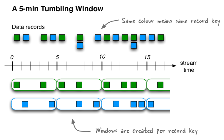
This diagram shows windowing a stream of data records with tumbling windows. Windows do not overlap because, by definition, the advance interval is identical to the window size. In this diagram the time numbers represent minutes; e.g., t=5 means “at the five-minute mark”. In reality, the unit of time in Kafka Streams is milliseconds, which means the time numbers would need to be multiplied with 60 * 1,000 to convert from minutes to milliseconds (e.g., t=5 would become t=300,000).
Tumbling time windows are aligned to the epoch, with the lower interval bound being inclusive and the upper bound being exclusive. “Aligned to the epoch” means that the first window starts at timestamp zero. For example, tumbling windows with a size of 5000ms have predictable window boundaries [0;5000),[5000;10000),... — and not[1000;6000),[6000;11000),... or even something “random” like [1452;6452),[6452;11452),....
The following code defines a tumbling window with a size of 5 minutes:
import java.time.Duration;
import org.apache.kafka.streams.kstream.TimeWindows;

// A tumbling time window with a size of 5 minutes (and, by definition, an implicit
// advance interval of 5 minutes).
Duration windowSizeMs = Duration.ofMinutes(5);
TimeWindows.of(windowSizeMs);

// The above is equivalent to the following code:
TimeWindows.of(windowSizeMs).advanceBy(windowSizeMs);
Counting example using tumbling windows:
// Key (String) is user ID, value (Avro record) is the page view event for that user.
// Such a data stream is often called a "clickstream".
KStream<String, GenericRecord> pageViews = ...;

// Count page views per window, per user, with tumbling windows of size 5 minutes
KTable<Windowed<String>, Long> windowedPageViewCounts = pageViews
    .groupByKey(Grouped.with(Serdes.String(), genericAvroSerde))
    .windowedBy(TimeWindows.of(Duration.ofMinutes(5)))
    .count();
Hopping time windows
Hopping time windows are windows based on time intervals. They model fixed-sized, (possibly) overlapping windows. A hopping window is defined by two properties: the window’s size and its advance interval (aka “hop”). The advance interval specifies by how much a window moves forward relative to the previous one. For example, you can configure a hopping window with a size 5 minutes and an advance interval of 1 minute. Since hopping windows can overlap – and in general they do – a data record may belong to more than one such window.
- Hopping windows vs. sliding windows
Hopping windows are sometimes called “sliding windows” in other stream processing tools. Kafka Streams follows the terminology in academic literature, where the semantics of sliding windows are different to those of hopping windows.
The following code defines a hopping window with a size of 5 minutes and an advance interval of 1 minute:
import java.time.Duration;
import org.apache.kafka.streams.kstream.TimeWindows;

// A hopping time window with a size of 5 minutes and an advance interval of 1 minute.
// The window's name -- the string parameter -- is used to e.g. name the backing state store.
Duration windowSizeMs = Duration.ofMinutes(5);
Duration advanceMs =    Duration.ofMinutes(1);
TimeWindows.of(windowSizeMs).advanceBy(advanceMs);
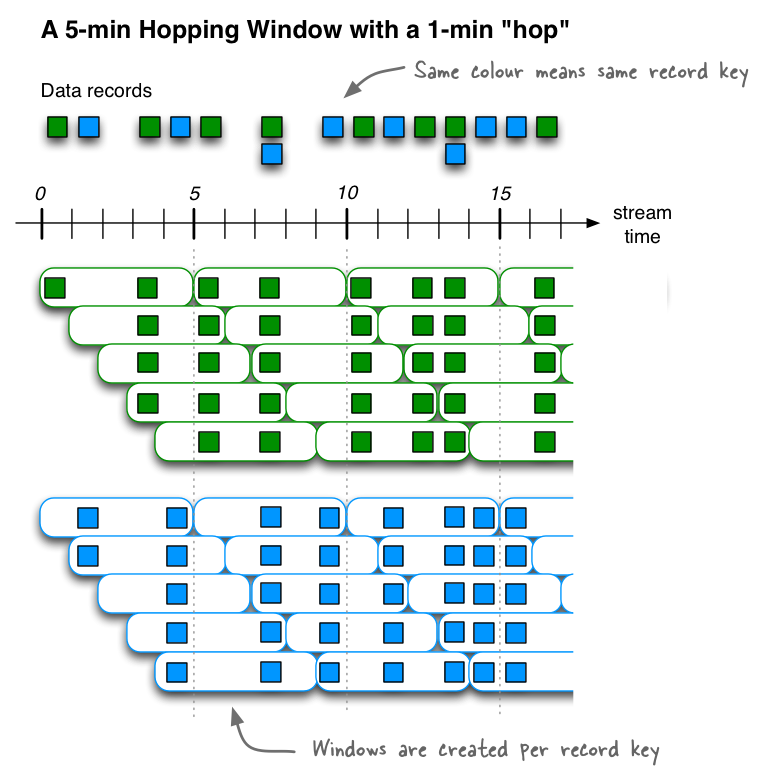
This diagram shows windowing a stream of data records with hopping windows. In this diagram the time numbers represent minutes; e.g., t=5 means “at the five-minute mark”. In reality, the unit of time in Kafka Streams is milliseconds, which means the time numbers would need to be multiplied with 60 * 1,000 to convert from minutes to milliseconds (e.g., t=5 would become t=300,000).
Hopping time windows are aligned to the epoch, with the lower interval bound being inclusive and the upper bound being exclusive. “Aligned to the epoch” means that the first window starts at timestamp zero. For example, hopping windows with a size of 5000ms and an advance interval (“hop”) of 3000ms have predictable window boundaries [0;5000),[3000;8000),... — and not [1000;6000),[4000;9000),... or even something “random” like [1452;6452),[4452;9452),....
Counting example using hopping windows:
// Key (String) is user ID, value (Avro record) is the page view event for that user.
// Such a data stream is often called a "clickstream".
KStream<String, GenericRecord> pageViews = ...;

// Count page views per window, per user, with hopping windows of size 5 minutes that advance every 1 minute
KTable<Windowed<String>, Long> windowedPageViewCounts = pageViews
    .groupByKey(Grouped.with(Serdes.String(), genericAvroSerde))
    .windowedBy(TimeWindows.of(Duration.ofMinutes(5).advanceBy(Duration.ofMinutes(1))))
    .count()
Unlike non-windowed aggregates that we have seen previously, windowed aggregates return a windowed KTable whose keys type is Windowed<K>. This is to differentiate aggregate values with the same key from different windows. The corresponding window instance and the embedded key can be retrieved as Windowed#window() and Windowed#key(), respectively.
Sliding time windows
Sliding windows differ significantly from hopping and tumbling windows. In Kafka Streams, sliding windows are used only for join operations, and can be using the JoinWindows class, and windowed aggregations, specified by using the SlidingWindows class.
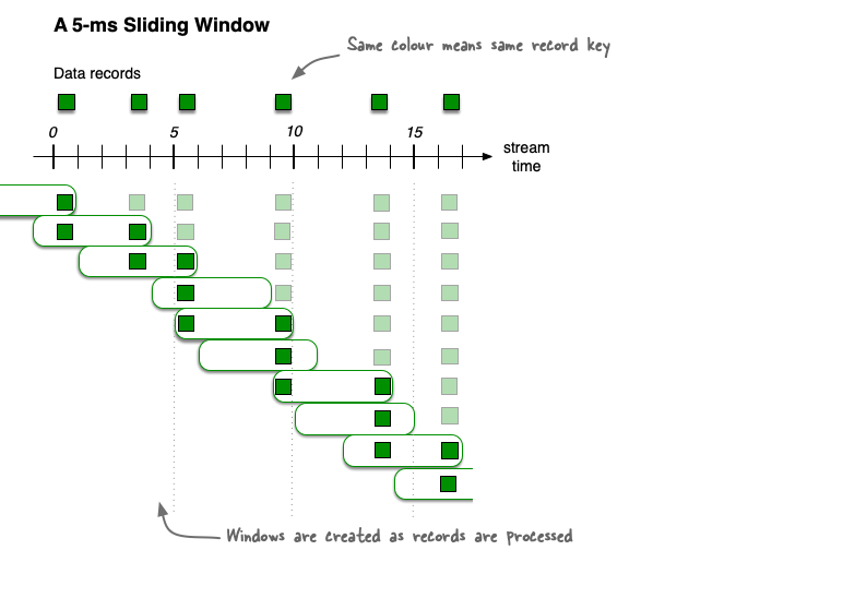
This diagram shows windowing a stream of data records with sliding windows. The overlap of the sliding window snapshots varies depending on the record times. In this diagram, the time numbers represent milliseconds. For example, t=5 means “at the five millisecond mark”.
A sliding window models a fixed-size window that slides continuously over the time axis. In this model, two data records are said to be included in the same window if (in the case of symmetric windows) the difference of their timestamps is within the window size. As a sliding window moves along the time axis, records may fall into multiple snapshots of the sliding window, but each unique combination of records appears only in one sliding window snapshot.
Sliding windows require that you set a grace period, as shown below. For time windows and session windows, setting the grace period is optional and defaults to 24 hours.
Sliding windows are aligned to the data record timestamps, not to the epoch. In contrast to hopping and tumbling windows, the lower and upper window time interval bounds of sliding windows are both inclusive.
The following code example defines a sliding window with a time difference of 10 minutes and a grace period of 30 minutes.
import org.apache.kafka.streams.kstream.SlidingWindows;

// A sliding time window with a time difference of 10 minutes
Duration windowTimeDifference = Duration.ofMinutes(10);
Duration grace = Duration.ofMinutes(30);

SlidingWindows.withTimeDifferenceAndGrace(windowTimeDifference, grace);
Session Windows
Session windows are used to aggregate key-based events into so-called sessions, the process of which is referred to as sessionization. Sessions represent a period of activity separated by a defined gap of inactivity (or “idleness”). Any events processed that fall within the inactivity gap of any existing sessions are merged into the existing sessions. If an event falls outside of the session gap, then a new session will be created.
Session windows are different from the other window types in that:
all windows are tracked independently across keys – e.g., windows of different keys typically have different start and end times
their window sizes sizes vary – even windows for the same key typically have different sizes
The prime area of application for session windows is user behavior analysis. Session-based analyses can range from simple metrics (e.g., count of user visits on a news website or social platform) to more complex metrics (e.g., customer conversion funnel and event flows).
The following code defines a session window with an inactivity gap of 5 minutes:
import java.time.Duration;
import org.apache.kafka.streams.kstream.SessionWindows;

// A session window with an inactivity gap of 5 minutes.
SessionWindows.with(Duration.ofMinutes(5));
Given the previous session window example, here’s what would happen on an input stream of six records. When the first three records arrive (upper part of in the diagram below), we’d have three sessions (see lower part) after having processed those records: two for the green record key, with one session starting and ending at the 0-minute mark (only due to the illustration it looks as if the session goes from 0 to 1), and another starting and ending at the 6-minute mark; and one session for the blue record key, starting and ending at the 2-minute mark.
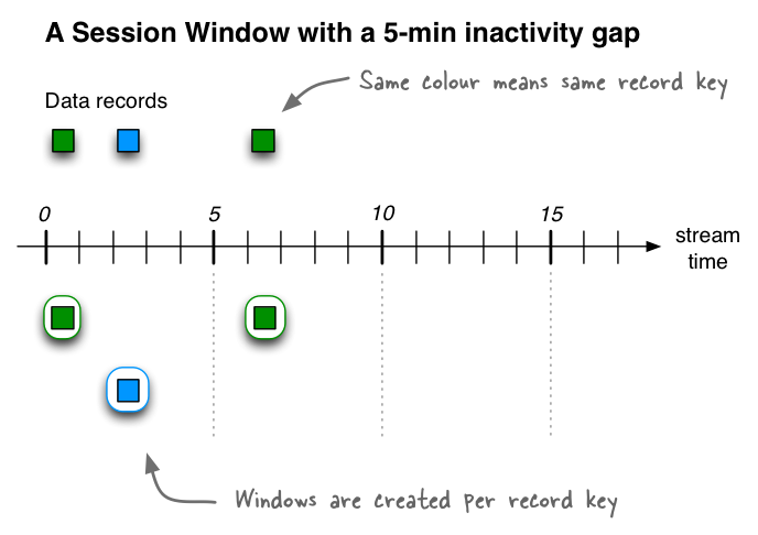
Detected sessions after having received three input records: two records for the green record key at t=0 and t=6, and one record for the blue record key at t=2. In this diagram the time numbers represent minutes; e.g., t=5 means “at the five-minute mark”. In reality, the unit of time in Kafka Streams is milliseconds, which means the time numbers would need to be multiplied with 60 * 1,000 to convert from minutes to milliseconds (e.g., t=5 would become t=300,000).
If we then receive three additional records (including two out-of-order records), what would happen is that the two existing sessions for the green record key will be merged into a single session starting at time 0 and ending at time 6, consisting of a total of three records. The existing session for the blue record key will be extended to end at time 5, consisting of a total of two records. And, finally, there will be a new session for the blue key starting and ending at time 11.
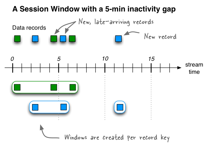
Detected sessions after having received six input records. Note the two out-of-order records at t=4 (green) and t=5 (blue), which lead to a merge of sessions and an extension of a session, respectively.
- Counting example using session windows
Assume you want to analyze reader behavior on a news website, like The New York Times, given a session definition of “As long as a person views (clicks on) another page at least once every 5 minutes (= inactivity gap), consider this to be a single visit and so a single, contiguous reading session for that person.” What you want to compute from this stream of input data is the number of page views per session.
// Key (String) is user ID, value (Avro record) is the page view event for that user.
// Such a data stream is often called a "clickstream".
KStream<String, GenericRecord> pageViews = ...;

// Count page views per session, per user, with session windows that have an inactivity gap of 5 minutes
KTable<Windowed<String>, Long> sessionizedPageViewCounts = pageViews
    .groupByKey(Grouped.with(Serdes.String(), genericAvroSerde))
    .windowedBy(SessionWindows.with(Duration.ofMinutes(5)))
    .count();
Window Final Results
In Kafka Streams, windowed computations update their results continuously. As new data arrives for a window, freshly computed results are emitted downstream. For many applications, this is ideal, since fresh results are always available, and Kafka Streams is designed to make programming continuous computations seamless. However, some applications need to take action only on the final result of a windowed computation. Common examples of this are sending alerts or delivering results to a system that doesn’t support updates.
Suppose that you have an hourly windowed count of events per user. If you want to send an alert when a user has less than three events in an hour, you have a real challenge. All users would match this condition at first, until they accrue enough events, so you can’t simply send an alert when someone matches the condition; you have to wait until you know you won’t see any more events for a particular window, and then send the alert.
Kafka Streams offers a clean way to define this logic: after defining your windowed computation, you can suppress the intermediate results, emitting the final count for each user when the window is closed.
For example:
KGroupedStream<UserId, Event> grouped = ...;
grouped
    .windowedBy(TimeWindows.of(Duration.ofHours(1)).grace(Duration.ofMinutes(10)))
    .count()
    .suppress(Suppressed.untilWindowCloses(unbounded()))
    .filter((windowedUserId, count) -> count < 3)
    .toStream()
    .foreach((windowedUserId, count) -> sendAlert(windowedUserId.window(), windowedUserId.key(), count));
The key parts of this program are:
grace(Duration.ofMinutes(10))This allows us to bound the unorder (or delay) of events the window will accept. For example, the 09:00 to 10:00 window will accept out-of-order records until 10:10, at which point, the window is closed.
.suppress(Suppressed.untilWindowCloses(...))This configures the suppression operator to emit nothing for a window until it closes, and then emit the final result. For example, if user
Ugets 10 events between 09:00 and 10:10, thefilterdownstream of the suppression will get no events for the windowed key@09:00-10:00until 10:10, and then it will get exactly one event with the value10. This is the final result of the windowed count.unbounded()This configures the buffer used for storing events until their windows close. Production code is able to put a cap on the amount of memory to use for the buffer, but this simple example creates a buffer with no upper bound.
One thing to note is that suppression is just like any other Kafka Streams operator, so you can build a topology with two branches emerging from the count, one suppressed, and one not, or even multiple differently configured suppressions. This enables you to apply suppressions where they are needed and otherwise rely on the default continuous update behavior.
For more detailed information, see the JavaDoc on the Suppressed config object and KIP-328.
Window duration and joins
After you change the window duration in a join operation, the state store segments are no longer valid, because the segment ranges and their corresponding IDs change.
Although this situation would resolve eventually when existing segments are dropped after a full grace-period range, your application misses join results until this happens.
If you don’t want to reset your internal topics after you change window duration, you can erase RocksDB and let it rebuild from the changelog. This approach won’t give you data older than the original grace period, but it does cause existing data joins to emit correctly.
Example: Custom time window
In addition to using the windows implementations provided with the Kafka Streams client library, you can extend the Java Windows abstract class to create custom time windows to suit your use cases.
To view a custom implementation of a daily window starting every day at 6pm, refer to streams/window example.
The example also shows a potential problem in dealing with time zones that have daylight savings time.
Applying processors (Processor API integration)
Beyond the aforementioned stateless and stateful transformations, you may also leverage the Processor API from the DSL. There are a number of scenarios where this may be helpful:
Customization: You need to implement special, customized logic that is not or not yet available in the DSL.
Combining ease-of-use with full flexibility where it’s needed: Even though you generally prefer to use the expressiveness of the DSL, there are certain steps in your processing that require more flexibility and tinkering than the DSL provides. For example, only the Processor API provides access to a record’s metadata such as its topic, partition, and offset information. However, you don’t want to switch completely to the Processor API just because of that.
Migrating from other tools: You are migrating from other stream processing technologies that provide an imperative API, and migrating some of your legacy code to the Processor API was faster and/or easier than to migrate completely to the DSL right away.
Operations and concepts
KStream#process: Process all records in a stream, one record at a time, by applying aProcessor(provided by a givenProcessorSupplier);KStream#processValues: Process all records in a stream, one record at a time, by applying aFixedKeyProcessor(provided by a givenFixedKeyProcessorSupplier);Processor: A processor of key-value pair records;ContextualProcessor: An abstract implementation ofProcessorthat manages theProcessorContextinstance.FixedKeyProcessor: A processor of key-value pair records where keys are immutable;ContextualFixedKeyProcessor: An abstract implementation ofFixedKeyProcessorthat manages theFixedKeyProcessorContextinstance.ProcessorSupplier: A processor supplier that can create one or moreProcessorinstances; andFixedKeyProcessorSupplier: A processor supplier that can create one or moreFixedKeyProcessorinstances.
Examples
The following examples show how to apply process and processValues to your Kafka Streams application.
Example | Operation | State Type |
|---|---|---|
process | Stateless | |
process | Stateful | |
processValues | Stateless | |
processValues | Stateful |
Categorize logs by severity
Idea: You have a stream of log messages. Each message contains a severity level, for example, INFO, WARN, ERROR, in the value. The processor filters messages, routing ERROR messages to a dedicated topic and discarding INFO messages. The rest (WARN) are forwarded to a dedicated topic too.
Real-world context: In a production monitoring system, categorizing logs by severity ensures ERROR logs are sent to a critical incident management system, WARN logs are analyzed for potential risks, and INFO logs are stored for basic reporting purposes.
public class CategorizingLogsBySeverityExample {
    private static final String ERROR_LOGS_TOPIC = "error-logs-topic";
    private static final String INPUT_LOGS_TOPIC = "input-logs-topic";
    private static final String UNKNOWN_LOGS_TOPIC = "unknown-logs-topic";
    private static final String WARN_LOGS_TOPIC = "warn-logs-topic";

    public static void categorizeWithProcess(final StreamsBuilder builder) {
        final KStream<String, String> logStream = builder.stream(INPUT_LOGS_TOPIC);
        logStream.process(LogSeverityProcessor::new)
                .to((key, value, recordContext) -> {
                    // Determine the target topic dynamically
                    if ("ERROR".equals(key)) return ERROR_LOGS_TOPIC;
                    if ("WARN".equals(key)) return WARN_LOGS_TOPIC;
                    return UNKNOWN_LOGS_TOPIC;
                });
    }

    private static class LogSeverityProcessor extends ContextualProcessor<String, String, String, String> {
        @Override
        public void process(final Record<String, String> record) {
            if (record.value() == null) {
                return; // Skip null values
            }

            // Assume the severity is the first word in the log message
            // For example: "ERROR: Disk not found" -> "ERROR"
            final int colonIndex = record.value().indexOf(':');
            final String severity = colonIndex > 0 ? record.value().substring(0, colonIndex).trim() : "UNKNOWN";

            // Route logs based on severity
            switch (severity) {
                case "ERROR":
                    context().forward(record.withKey(ERROR_LOGS_TOPIC));
                    break;
                case "WARN":
                    context().forward(record.withKey(WARN_LOGS_TOPIC));
                    break;
                case "INFO":
                    // INFO logs are ignored
                    break;
                default:
                    // Forward to an "unknown" topic for logs with unrecognized severities
                    context().forward(record.withKey(UNKNOWN_LOGS_TOPIC));
            }
        }
    }
}
Cumulative discounts for a loyalty program
Idea: A stream of purchase events contains user IDs and transaction amounts. Use a state store to accumulate the total spending of each user. When their total crosses a threshold, apply a discount on their next transaction and update their accumulated total.
Real-world context: In a retail loyalty program, tracking cumulative customer spending enables dynamic rewards, such as issuing a discount when a customer’s total purchases exceed a predefined limit.
public class CumulativeDiscountsForALoyaltyProgramExample {
    private static final double DISCOUNT_THRESHOLD = 100.0;
    private static final String CUSTOMER_SPENDING_STORE = "customer-spending-store";
    private static final String DISCOUNT_NOTIFICATION_MESSAGE =
            "Discount applied! You have received a reward for your purchases.";
    private static final String DISCOUNT_NOTIFICATIONS_TOPIC = "discount-notifications-topic";
    private static final String PURCHASE_EVENTS_TOPIC = "purchase-events-topic";

    public static void applyDiscountWithProcess(final StreamsBuilder builder) {
        // Define the state store for tracking cumulative spending
        builder.addStateStore(
                Stores.keyValueStoreBuilder(
                        Stores.inMemoryKeyValueStore(CUSTOMER_SPENDING_STORE),
                        Serdes.String(),
                        Serdes.Double()
                )
        );
        final KStream<String, Double> purchaseStream = builder.stream(PURCHASE_EVENTS_TOPIC);
        // Apply the Processor with the state store
        final KStream<String, String> notificationStream =
                purchaseStream.process(CumulativeDiscountProcessor::new, CUSTOMER_SPENDING_STORE);
        // Send the notifications to the output topic
        notificationStream.to(DISCOUNT_NOTIFICATIONS_TOPIC);
    }

    private static class CumulativeDiscountProcessor implements Processor<String, Double, String, String> {
        private KeyValueStore<String, Double> spendingStore;
        private ProcessorContext<String, String> context;

        @Override
        public void init(final ProcessorContext<String, String> context) {
            this.context = context;
            // Retrieve the state store for cumulative spending
            spendingStore = context.getStateStore(CUSTOMER_SPENDING_STORE);
        }

        @Override
        public void process(final Record<String, Double> record) {
            if (record.value() == null) {
                return; // Skip null purchase amounts
            }

            // Get the current spending total for the customer
            Double currentSpending = spendingStore.get(record.key());
            if (currentSpending == null) {
                currentSpending = 0.0;
            }
            // Update the cumulative spending
            currentSpending += record.value();
            spendingStore.put(record.key(), currentSpending);

            // Check if the customer qualifies for a discount
            if (currentSpending >= DISCOUNT_THRESHOLD) {
                // Reset the spending after applying the discount
                spendingStore.put(record.key(), currentSpending - DISCOUNT_THRESHOLD);
                // Send a discount notification
                context.forward(record.withValue(DISCOUNT_NOTIFICATION_MESSAGE));
            }
        }
    }
}
Replace slang in text messages
Idea: A messaging stream contains user-generated content, and you want to replace slang words with their formal equivalents, for example, “u” becomes “you”, “brb” becomes “be right back”. The operation modifies only the message value and keeps the key intact.
Real-World Context: In customer support chat systems, normalizing text by replacing slang with formal equivalents ensures that automated sentiment analysis tools work accurately and provide reliable insights.
public class ReplacingSlangTextInMessagesExample {
    private static final Map<String, String> SLANG_DICTIONARY = Map.of(
            "u", "you",
            "brb", "be right back",
            "omg", "oh my god",
            "btw", "by the way"
    );
    private static final String INPUT_MESSAGES_TOPIC = "input-messages-topic";
    private static final String OUTPUT_MESSAGES_TOPIC = "output-messages-topic";

    public static void replaceWithProcessValues(final StreamsBuilder builder) {
        KStream<String, String> messageStream = builder.stream(INPUT_MESSAGES_TOPIC);
        messageStream.processValues(SlangReplacementProcessor::new).to(OUTPUT_MESSAGES_TOPIC);
    }

    private static class SlangReplacementProcessor extends ContextualFixedKeyProcessor<String, String, String> {
        @Override
        public void process(final FixedKeyRecord<String, String> record) {
            if (record.value() == null) {
                return; // Skip null values
            }

            // Replace slang words in the message
            final String[] words = record.value().split("\\s+");
            for (final String word : words) {
                String replacedWord = SLANG_DICTIONARY.getOrDefault(word, word);
                context().forward(record.withValue(replacedWord));
            }
        }
    }
}
Traffic radar monitoring car count
Idea: A radar monitors cars passing along a road stretch. A system counts the cars for each day, maintaining a cumulative total for the current day in a state store. At the end of the day, the count is emitted and the state is cleared for the next day.
Real-world context: A car counting system can be useful for determining measures for widening or controlling traffic depending on the number of cars passing through the monitored stretch.
public class TrafficRadarMonitoringCarCountExample {
    private static final String DAILY_COUNT_STORE = "price-state-store";
    private static final String DAILY_COUNT_TOPIC = "price-state-topic";
    private static final String RADAR_COUNT_TOPIC = "car-radar-topic";

    public static void countWithProcessValues(final StreamsBuilder builder) {
        // Define a state store for tracking daily car counts
        builder.addStateStore(
                Stores.keyValueStoreBuilder(
                        Stores.inMemoryKeyValueStore(DAILY_COUNT_STORE),
                        Serdes.String(),
                        Serdes.Long()
                )
        );
        final KStream<Void, String> radarStream = builder.stream(RADAR_COUNT_TOPIC);
        // Apply the FixedKeyProcessor with the state store
        radarStream.processValues(DailyCarCountProcessor::new, DAILY_COUNT_STORE)
                .to(DAILY_COUNT_TOPIC);
    }

    private static class DailyCarCountProcessor implements FixedKeyProcessor<Void, String, String> {
        private FixedKeyProcessorContext<Void, String> context;
        private KeyValueStore<String, Long> stateStore;
        private static final DateTimeFormatter DATE_FORMATTER =
                DateTimeFormatter.ofPattern("yyyy-MM-dd").withZone(ZoneId.systemDefault());

        @Override
        public void init(final FixedKeyProcessorContext<Void, String> context) {
            this.context = context;
            stateStore = context.getStateStore(DAILY_COUNT_STORE);
        }

        @Override
        public void process(final FixedKeyRecord<Void, String> record) {
            if (record.value() == null) {
                return; // Skip null events
            }

            // Derive the current day from the event timestamp
            final long timestamp = System.currentTimeMillis(); // Use system time for simplicity
            final String currentDay = DATE_FORMATTER.format(Instant.ofEpochMilli(timestamp));
            // Retrieve the current count for the day
            Long dailyCount = stateStore.get(currentDay);
            if (dailyCount == null) {
                dailyCount = 0L;
            }
            // Increment the count
            dailyCount++;
            stateStore.put(currentDay, dailyCount);

            // Emit the current day's count
            context.forward(record.withValue(String.format("Day: %s, Car Count: %s", currentDay, dailyCount)));
        }
    }
}
Keynotes
Type safety and flexibility: The
processandprocessValuesAPIs utilizeProcessorContextandRecordorFixedKeyRecordobjects for better type safety and flexibility of custom processing logic.Clear state and logic management: Implementations for
ProcessororFixedKeyProcessorshould manage state and logic clearly. Usecontext().forward()for emitting records downstream.Unified API: Consolidates multiple methods into a single, versatile API.
Future-Proof: Ensures compatibility with the latest Kafka Streams releases.
Transformers removal and migration to processors
As of Kafka 4.0, several deprecated methods in the Kafka Streams API, such as transform, flatTransform, transformValues, flatTransformValues, and process have been removed. These methods have been replaced with the more versatile Processor API. This guide provides detailed steps for migrating existing code to use the new Processor API and explains the benefits of the changes.
The following deprecated methods are no longer available in Kafka Streams:
KStream#transformKStream#flatTransformKStream#transformValuesKStream#flatTransformValuesKStream#process
The Processor API now serves as a unified replacement for all these methods. It simplifies the API surface while maintaining support for both stateless and stateful operations.
Migration examples
To migrate from the deprecated transform, transformValues, flatTransform, and flatTransformValues methods to the Processor API (PAPI) in Kafka Streams, let’s resume the previous examples. The new process and processValues methods enable a more flexible and reusable approach by requiring implementations of the Processor or FixedKeyProcessor interfaces.
Example | Migrating from | Migrating to | State Type |
|---|---|---|---|
|
| Stateless | |
|
| Stateful | |
|
| Stateless | |
|
| Stateful |
Categorize logs by severity
In the following code example, the categorizeWithFlatTransform and categorizeWithProcess methods show how you can migrate from flatTransform to process.
public class CategorizingLogsBySeverityExample {
    private static final String ERROR_LOGS_TOPIC = "error-logs-topic";
    private static final String INPUT_LOGS_TOPIC = "input-logs-topic";
    private static final String UNKNOWN_LOGS_TOPIC = "unknown-logs-topic";
    private static final String WARN_LOGS_TOPIC = "warn-logs-topic";

    public static void categorizeWithFlatTransform(final StreamsBuilder builder) {
        final KStream<String, String> logStream = builder.stream(INPUT_LOGS_TOPIC);
        logStream.flatTransform(LogSeverityTransformer::new)
                .to((key, value, recordContext) -> {
                    // Determine the target topic dynamically
                    if ("ERROR".equals(key)) return ERROR_LOGS_TOPIC;
                    if ("WARN".equals(key)) return WARN_LOGS_TOPIC;
                    return UNKNOWN_LOGS_TOPIC;
                });
    }

    public static void categorizeWithProcess(final StreamsBuilder builder) {
        final KStream<String, String> logStream = builder.stream(INPUT_LOGS_TOPIC);
        logStream.process(LogSeverityProcessor::new)
                .to((key, value, recordContext) -> {
                    // Determine the target topic dynamically
                    if ("ERROR".equals(key)) return ERROR_LOGS_TOPIC;
                    if ("WARN".equals(key)) return WARN_LOGS_TOPIC;
                    return UNKNOWN_LOGS_TOPIC;
                });
    }

    private static class LogSeverityTransformer implements Transformer<String, String, Iterable<KeyValue<String, String>>> {
        @Override
        public void init(org.apache.kafka.streams.processor.ProcessorContext context) {
        }

        @Override
        public Iterable<KeyValue<String, String>> transform(String key, String value) {
            if (value == null) {
                return Collections.emptyList(); // Skip null values
            }

            // Assume the severity is the first word in the log message
            // For example: "ERROR: Disk not found" -> "ERROR"
            int colonIndex = value.indexOf(':');
            String severity = colonIndex > 0 ? value.substring(0, colonIndex).trim() : "UNKNOWN";

            // Create appropriate KeyValue pair based on severity
            return switch (severity) {
                case "ERROR" -> List.of(new KeyValue<>("ERROR", value));
                case "WARN" -> List.of(new KeyValue<>("WARN", value));
                case "INFO" -> Collections.emptyList(); // INFO logs are ignored
                default -> List.of(new KeyValue<>("UNKNOWN", value));
            };
        }

        @Override
        public void close() {
        }
    }

    private static class LogSeverityProcessor extends ContextualProcessor<String, String, String, String> {
        @Override
        public void process(final Record<String, String> record) {
            if (record.value() == null) {
                return; // Skip null values
            }

            // Assume the severity is the first word in the log message
            // For example: "ERROR: Disk not found" -> "ERROR"
            final int colonIndex = record.value().indexOf(':');
            final String severity = colonIndex > 0 ? record.value().substring(0, colonIndex).trim() : "UNKNOWN";

            // Route logs based on severity
            switch (severity) {
                case "ERROR":
                    context().forward(record.withKey(ERROR_LOGS_TOPIC));
                    break;
                case "WARN":
                    context().forward(record.withKey(WARN_LOGS_TOPIC));
                    break;
                case "INFO":
                    // INFO logs are ignored
                    break;
                default:
                    // Forward to an "unknown" topic for logs with unrecognized severities
                    context().forward(record.withKey(UNKNOWN_LOGS_TOPIC));
            }
        }
    }
}
Cumulative discounts for a loyalty program
In the following code example, the applyDiscountWithTransform and applyDiscountWithProcess methods show how you can migrate from transform to process.
public class CumulativeDiscountsForALoyaltyProgramExample {
    private static final double DISCOUNT_THRESHOLD = 100.0;
    private static final String CUSTOMER_SPENDING_STORE = "customer-spending-store";
    private static final String DISCOUNT_NOTIFICATION_MESSAGE =
            "Discount applied! You have received a reward for your purchases.";
    private static final String DISCOUNT_NOTIFICATIONS_TOPIC = "discount-notifications-topic";
    private static final String PURCHASE_EVENTS_TOPIC = "purchase-events-topic";

    public static void applyDiscountWithTransform(final StreamsBuilder builder) {
        // Define the state store for tracking cumulative spending
        builder.addStateStore(
                Stores.keyValueStoreBuilder(
                        Stores.inMemoryKeyValueStore(CUSTOMER_SPENDING_STORE),
                        Serdes.String(),
                        Serdes.Double()
                )
        );
        final KStream<String, Double> purchaseStream = builder.stream(PURCHASE_EVENTS_TOPIC);
        // Apply the Transformer with the state store
        final KStream<String, String> notificationStream =
                purchaseStream.transform(CumulativeDiscountTransformer::new, CUSTOMER_SPENDING_STORE);
        // Send the notifications to the output topic
        notificationStream.to(DISCOUNT_NOTIFICATIONS_TOPIC);
    }

    public static void applyDiscountWithProcess(final StreamsBuilder builder) {
        // Define the state store for tracking cumulative spending
        builder.addStateStore(
                Stores.keyValueStoreBuilder(
                        Stores.inMemoryKeyValueStore(CUSTOMER_SPENDING_STORE),
                        org.apache.kafka.common.serialization.Serdes.String(),
                        org.apache.kafka.common.serialization.Serdes.Double()
                )
        );
        final KStream<String, Double> purchaseStream = builder.stream(PURCHASE_EVENTS_TOPIC);
        // Apply the Processor with the state store
        final KStream<String, String> notificationStream =
                purchaseStream.process(CumulativeDiscountProcessor::new, CUSTOMER_SPENDING_STORE);
        // Send the notifications to the output topic
        notificationStream.to(DISCOUNT_NOTIFICATIONS_TOPIC);
    }

    private static class CumulativeDiscountTransformer implements Transformer<String, Double, KeyValue<String, String>> {
        private KeyValueStore<String, Double> spendingStore;

        @Override
        public void init(final org.apache.kafka.streams.processor.ProcessorContext context) {
            // Retrieve the state store for cumulative spending
            spendingStore = context.getStateStore(CUSTOMER_SPENDING_STORE);
        }

        @Override
        public KeyValue<String, String> transform(final String key, final Double value) {
            if (value == null) {
                return null; // Skip null purchase amounts
            }

            // Get the current spending total for the customer
            Double currentSpending = spendingStore.get(key);
            if (currentSpending == null) {
                currentSpending = 0.0;
            }
            // Update the cumulative spending
            currentSpending += value;
            spendingStore.put(key, currentSpending);

            // Check if the customer qualifies for a discount
            if (currentSpending >= DISCOUNT_THRESHOLD) {
                // Reset the spending after applying the discount
                spendingStore.put(key, currentSpending - DISCOUNT_THRESHOLD);
                // Return a notification message
                return new KeyValue<>(key, DISCOUNT_NOTIFICATION_MESSAGE);
            }
            return null; // No discount, so no output for this record
        }

        @Override
        public void close() {
        }
    }

    private static class CumulativeDiscountProcessor implements Processor<String, Double, String, String> {
        private KeyValueStore<String, Double> spendingStore;
        private ProcessorContext<String, String> context;

        @Override
        public void init(final ProcessorContext<String, String> context) {
            this.context = context;
            // Retrieve the state store for cumulative spending
            spendingStore = context.getStateStore(CUSTOMER_SPENDING_STORE);
         }

        @Override
        public void process(final Record<String, Double> record) {
            if (record.value() == null) {
                return; // Skip null purchase amounts
            }

            // Get the current spending total for the customer
            Double currentSpending = spendingStore.get(record.key());
            if (currentSpending == null) {
                currentSpending = 0.0;
            }
            // Update the cumulative spending
            currentSpending += record.value();
            spendingStore.put(record.key(), currentSpending);

            // Check if the customer qualifies for a discount
            if (currentSpending >= DISCOUNT_THRESHOLD) {
                // Reset the spending after applying the discount
                spendingStore.put(record.key(), currentSpending - DISCOUNT_THRESHOLD);
                // Send a discount notification
                context.forward(record.withValue(DISCOUNT_NOTIFICATION_MESSAGE));
            }
        }
    }
}
Replace slang in text messages
In the following code example, the replaceWithFlatTransformValues and replaceWithProcessValues methods show how you can migrate from flatTransformValues to processValues.
public class ReplacingSlangTextInMessagesExample {
    private static final Map<String, String> SLANG_DICTIONARY = Map.of(
            "u", "you",
            "brb", "be right back",
            "omg", "oh my god",
            "btw", "by the way"
    );
    private static final String INPUT_MESSAGES_TOPIC = "input-messages-topic";
    private static final String OUTPUT_MESSAGES_TOPIC = "output-messages-topic";

    public static void replaceWithFlatTransformValues(final StreamsBuilder builder) {
        KStream<String, String> messageStream = builder.stream(INPUT_MESSAGES_TOPIC);
        messageStream.flatTransformValues(SlangReplacementTransformer::new).to(OUTPUT_MESSAGES_TOPIC);
    }

    public static void replaceWithProcessValues(final StreamsBuilder builder) {
        KStream<String, String> messageStream = builder.stream(INPUT_MESSAGES_TOPIC);
        messageStream.processValues(SlangReplacementProcessor::new).to(OUTPUT_MESSAGES_TOPIC);
    }

    private static class SlangReplacementTransformer implements ValueTransformer<String, Iterable<String>> {

        @Override
        public void init(final org.apache.kafka.streams.processor.ProcessorContext context) {
        }

        @Override
        public Iterable<String> transform(final String value) {
            if (value == null) {
                return Collections.emptyList(); // Skip null values
            }

            // Replace slang words in the message
            final String[] words = value.split("\\s+");
            return Arrays.asList(
                    Arrays.stream(words)
                            .map(word -> SLANG_DICTIONARY.getOrDefault(word, word))
                            .toArray(String[]::new)
            );
        }

        @Override
        public void close() {
        }
    }

    private static class SlangReplacementProcessor extends ContextualFixedKeyProcessor<String, String, String> {
        @Override
        public void process(final FixedKeyRecord<String, String> record) {
            if (record.value() == null) {
                return; // Skip null values
            }

            // Replace slang words in the message
            final String[] words = record.value().split("\\s+");
            for (final String word : words) {
                String replacedWord = SLANG_DICTIONARY.getOrDefault(word, word);
                context().forward(record.withValue(replacedWord));
            }
        }
    }
}
Traffic radar monitoring car count
In the following code example, the countWithTransformValues and countWithProcessValues methods show how you can migrate from transformValues to processValues.
public class TrafficRadarMonitoringCarCountExample {
    private static final String DAILY_COUNT_STORE = "price-state-store";
    private static final String DAILY_COUNT_TOPIC = "price-state-topic";
    private static final String RADAR_COUNT_TOPIC = "car-radar-topic";

    public static void countWithTransformValues(final StreamsBuilder builder) {
        // Define a state store for tracking daily car counts
        builder.addStateStore(
                Stores.keyValueStoreBuilder(
                        Stores.inMemoryKeyValueStore(DAILY_COUNT_STORE),
                        org.apache.kafka.common.serialization.Serdes.String(),
                        org.apache.kafka.common.serialization.Serdes.Long()
                )
        );
        final KStream<Void, String> radarStream = builder.stream(RADAR_COUNT_TOPIC);
        // Apply the ValueTransformer with the state store
        radarStream.transformValues(DailyCarCountTransformer::new, DAILY_COUNT_STORE)
                .to(DAILY_COUNT_TOPIC);
    }

    public static void countWithProcessValues(final StreamsBuilder builder) {
        // Define a state store for tracking daily car counts
        builder.addStateStore(
                Stores.keyValueStoreBuilder(
                        Stores.inMemoryKeyValueStore(DAILY_COUNT_STORE),
                        org.apache.kafka.common.serialization.Serdes.String(),
                        org.apache.kafka.common.serialization.Serdes.Long()
                )
        );
        final KStream<Void, String> radarStream = builder.stream(RADAR_COUNT_TOPIC);
        // Apply the FixedKeyProcessor with the state store
        radarStream.processValues(DailyCarCountProcessor::new, DAILY_COUNT_STORE)
                .to(DAILY_COUNT_TOPIC);
    }

    private static class DailyCarCountTransformer implements ValueTransformerWithKey<Void, String, String> {
        private KeyValueStore<String, Long> stateStore;
        private static final DateTimeFormatter DATE_FORMATTER =
                DateTimeFormatter.ofPattern("yyyy-MM-dd").withZone(ZoneId.systemDefault());

        @Override
        public void init(final org.apache.kafka.streams.processor.ProcessorContext context) {
            // Access the state store
            stateStore = context.getStateStore(DAILY_COUNT_STORE);
        }

        @Override
        public String transform(Void readOnlyKey, String value) {
            if (value == null) {
                return null; // Skip null events
            }

            // Derive the current day from the event timestamp
            final long timestamp = System.currentTimeMillis(); // Use system time for simplicity
            final String currentDay = DATE_FORMATTER.format(Instant.ofEpochMilli(timestamp));
            // Retrieve the current count for the day
            Long dailyCount = stateStore.get(currentDay);
            if (dailyCount == null) {
                dailyCount = 0L;
            }
            // Increment the count
            dailyCount++;
            stateStore.put(currentDay, dailyCount);

            // Return the current day's count
            return String.format("Day: %s, Car Count: %s", currentDay, dailyCount);
        }

        @Override
        public void close() {
        }
    }

    private static class DailyCarCountProcessor implements FixedKeyProcessor<Void, String, String> {
        private FixedKeyProcessorContext<Void, String> context;
        private KeyValueStore<String, Long> stateStore;
        private static final DateTimeFormatter DATE_FORMATTER =
                DateTimeFormatter.ofPattern("yyyy-MM-dd").withZone(ZoneId.systemDefault());

        @Override
        public void init(final FixedKeyProcessorContext<Void, String> context) {
            this.context = context;
            stateStore = context.getStateStore(DAILY_COUNT_STORE);
        }

        @Override
        public void process(final FixedKeyRecord<Void, String> record) {
            if (record.value() == null) {
                return; // Skip null events
            }

            // Derive the current day from the event timestamp
            final long timestamp = System.currentTimeMillis(); // Use system time for simplicity
            final String currentDay = DATE_FORMATTER.format(Instant.ofEpochMilli(timestamp));
            // Retrieve the current count for the day
            Long dailyCount = stateStore.get(currentDay);
            if (dailyCount == null) {
                dailyCount = 0L;
            }
            // Increment the count
            dailyCount++;
            stateStore.put(currentDay, dailyCount);

            // Emit the current day's count
            context.forward(record.withValue(String.format("Day: %s, Car Count: %s", currentDay, dailyCount)));
        }
    }
}
Removal of old process method
In addition to the methods mentioned previously, the process method, which integrated the ‘old’ Processor API, that is, Processor as opposed to the new api.Processor, into the DSL, has also been removed. The following example shows how to migrate to the new process.
Example
Idea: The system monitors page views for a website in real-time. When a page reaches a predefined popularity threshold, for example, 1000 views, the system sends an email alert automatically to the site administrator or marketing team to notify them of the page’s success. This helps teams quickly identify high-performing content and act on it, such as promoting the page further or analyzing the traffic source.
Real-world context: In a content management system (CMS) for a news or blogging platform, it’s crucial to track the popularity of articles or posts. For example:
Marketing teams: Use the notification to highlight trending content on social media or email newsletters.
Operations teams: Use the alert to ensure the site can handle increased traffic for popular pages.
Ad managers: Identify pages where additional ad placements might maximize revenue.
By automating the detection of popular pages, the system eliminates the need for manual monitoring and ensures timely actions to capitalize on the content’s performance.
public class PopularPageEmailAlertExample {
    private static final String ALERTS_EMAIL = "alerts@yourcompany.com";
    private static final String PAGE_VIEWS_TOPIC = "page-views-topic";

    public static void alertWithOldProcess(StreamsBuilder builder) {
        KStream<String, Long> pageViews = builder.stream(PAGE_VIEWS_TOPIC);
        // Filter pages with exactly 1000 views and process them using the old API
        pageViews.filter((pageId, viewCount) -> viewCount == 1000)
                .process(PopularPageEmailAlertOld::new);
    }

    public static void alertWithNewProcess(StreamsBuilder builder) {
        KStream<String, Long> pageViews = builder.stream(PAGE_VIEWS_TOPIC);
        // Filter pages with exactly 1000 views and process them using the new API
        pageViews.filter((pageId, viewCount) -> viewCount == 1000)
                .process(PopularPageEmailAlertNew::new);
    }

    private static class PopularPageEmailAlertOld extends AbstractProcessor<String, Long> {
        @Override
        public void init(org.apache.kafka.streams.processor.ProcessorContext context) {
            super.init(context);
            System.out.println("Initialized email client for: " + ALERTS_EMAIL);
        }

        @Override
        public void process(String key, Long value) {
            if (value == null) return;

            if (value == 1000) {
                // Send an email alert
                System.out.printf("ALERT (Old API): Page %s has reached 1000 views. Sending email to %s%n", key, ALERTS_EMAIL);
            }
        }

        @Override
        public void close() {
            System.out.println("Tearing down email client for: " + ALERTS_EMAIL);
        }
    }

    private static class PopularPageEmailAlertNew implements Processor<String, Long, Void, Void> {
        @Override
        public void init(ProcessorContext<Void, Void> context) {
            System.out.println("Initialized email client for: " + ALERTS_EMAIL);
        }

        @Override
        public void process(Record<String, Long> record) {
            if (record.value() == null) return;

            if (record.value() == 1000) {
                // Send an email alert
                System.out.printf("ALERT (New API): Page %s has reached 1000 views. Sending email to %s%n", record.key(), ALERTS_EMAIL);
            }
        }

        @Override
        public void close() {
            System.out.println("Tearing down email client for: " + ALERTS_EMAIL);
        }
    }
}
Name operators in a Kafka Streams DSL application
Kafka Streams enables you to name processors created by using the Streams DSL.
Control KTable emit rate
A KTable is logically a continuously updated table. These updates make their way to downstream operators whenever new data is available, ensuring that the whole computation is as fresh as possible. Most programs describe a series of logical transformations, and the update rate is not a factor in the program behavior.
In these cases, the rate of update is a performance concern, which is best addressed directly via the relevant configurations.
However, for some applications, the rate of update itself is an important semantic property.
Rather than achieving this as a side-effect of the record caches, you can directly impose a rate limit via the KTable#suppress operator.
For example:
KGroupedTable<String, String> groupedTable = ...;
groupedTable
    .count()
    .suppress(untilTimeLimit(Duration.ofMinutes(5), maxBytes(1_000_000L).emitEarlyWhenFull()))
    .toStream();
This configuration ensures that, downstream of suppress, each key is updated no more than once every 5 minutes (in stream time, not wall-clock time).
Note that the latest state for each key has to be buffered in memory for that 5-minute period. You have the option to control the maximum amount of memory to use for this buffer (in this case, 1MB). There is also an option to impose a limit in terms of number of records or to leave both limits unspecified.
Additionally, it is possible to choose what happens if the buffer fills up. This example takes a relaxed approach and just emits the oldest records before their 5-minute time limit to bring the buffer back down to size. Alternatively, you can choose to stop processing and shut the application down. This may seem extreme, but it gives you a guarantee that the 5-minute time limit will be absolutely enforced. After the application shuts down, you could allocate more memory for the buffer and resume processing. Emitting early is preferable for most applications.
For more detailed information, see the JavaDoc on the Suppressed config object and KIP-328.
Timestamp-based semantics for table processors
By default, tables in Kafka Streams use offset-based semantics. When multiple records arrive for the same key, the one with the largest record offset is considered the latest record for the key and is the record that appears in aggregation and join results computed on the table. This is true even in the event of out-of-order data. The record with the largest offset is considered to be the latest record for the key, even if this record does not have the largest timestamp.
An alternative to offset-based semantics is timestamp-based semantics. With timestamp-based semantics, the record with the largest timestamp is considered the latest record, even if there is another record with a larger offset (and smaller timestamp). If there is no out-of-order data (per key), then offset-based semantics and timestamp-based semantics are equivalent; the difference appears only when there is out-of-order data.
Starting with Confluent Platform 7.5 (Kafka Streams 3.5), Kafka Streams supports timestamp-based semantics through the use of versioned state stores. When a table is materialized with a versioned state store, it is a versioned table and results in different processor semantics in the presence of out-of-order data.
When performing a stream-table join, stream-side records join with the latest-by-timestamp table record which has a timestamp less than or equal to the stream record’s timestamp. This is in contrast to joining a stream to an unversioned table, in which case the latest-by-offset table record is joined, even if the stream-side record is out-of-order and has a lower timestamp.
Aggregations computed on the table include the latest-by-timestamp record for each key, instead of the latest-by-offset record. Out-of-order updates (per key) don’t trigger a new aggregation result. This is true for
countandreduceoperations as well, in addition toaggregateoperations.Table joins use the latest-by-timestamp record for each key, instead of the latest-by-offset record. Out-of-order updates (per key) don’t trigger a new join result. This is true for both primary-key table-table joins and also foreign-key table-table joins. If a versioned table is joined with an unversioned table, the result is the join of the latest-by-timestamp record from the versioned table with the latest-by-offset record from the unversioned table.
Table filter operations no longer suppress consecutive tombstones, so you may observe more
nullrecords downstream of the filter than when you filter an unversioned table. This is done to preserve a complete version history downstream, in the event of out-of-order data.
Once a table is materialized with a versioned store, downstream tables are also considered versioned until any of the following occurs:
A downstream table is materialized explicitly, either with an unversioned store supplier or with no store supplier. All stores are unversioned by default, including the default store supplier.
Any stateful transformation occurs, including aggregations and joins.
A table is converted to a stream and back.
The results of certain processors should not be materialized with versioned stores, as these processors don’t produce a complete older version history and therefore materialization as a versioned table leads to unpredictable results:
Aggregate processors, for both table and stream aggregations. This includes
aggregate,count, andreduceoperations.Table-table join processors, including both primary-key and foreign-key joins.
For more information, see Versioned key-value state stores.
Writing streams back to Kafka
Any streams and tables may be (continuously) written back to a Kafka topic. As described in more detail below, the output data might be re-partitioned on its way to Kafka, depending on the situation.
Writing to Kafka | Description | |
|---|---|
To
| Terminal operation. Write the records to Kafka topic(s). (KStream details) When to provide serdes explicitly:
A variant of Another variant of KStream<String, Long> stream = ...;
KTable<String, Long> table = ...;
// Write the stream to the output topic, using the configured default key
// and value serdes of your `StreamsConfig`.
stream.to("my-stream-output-topic");
// Write the stream to the output topic, using explicit key and value serdes,
// (thus overriding the defaults of your `StreamsConfig`).
stream.to("my-stream-output-topic", Produced.with(Serdes.String(), Serdes.Long());
// Write the stream to the output topics. The topic name is determined dynamically for
// each record; also use explicit stream partitioner to determine which partition
// of the topic to send to.
stream.to(
(key, value, recordContext) -> // topicNameExtractor
if (myPattern.matcher(key).matches) {
"special-stream-output-topic"
} else {
"normal-stream-output-topic"
},
Produced.streamPartitioner(
(topic, key, value, numPartitions) ->
if (topic.equals("special-stream-output-topic")) {
specialHash(key, value, numPartitions)
} else {
md5Hash(key, value, numPartitions)
}
)
);
Causes data re-partitioning if any of the following conditions is true:
|
- When you want to write to systems other than Kafka
Beside writing the data back to Kafka, you can also apply a custom processor as a stream sink at the end of the processing, for example, to write to external databases.
Doing this is not a recommended pattern, and Confluent suggests using the Kafka Connect API instead. But if you do use such a sink processor, be aware that it’s your responsibility to guarantee message delivery semantics when communicating with such external systems, for example, to retry on delivery failure or to prevent message duplication.
Kafka Streams DSL for Scala
Kafka Streams provides a Scala wrapper for the Java API to provide:
Better type inference in Scala.
Less boilerplate in application code.
The usual builder-style composition that developers get with the original Java API.
Implicit serializers and de-serializers leading to better abstraction and less verbosity.
Better type safety during compile time.
All functionality provided by Kafka Streams DSL for Scala are under the root package name of org.apache.kafka.streams.scala.
Many of the public facing types from the Java API are wrapped. The following Scala abstractions are available to the user:
org.apache.kafka.streams.scala.StreamsBuilderorg.apache.kafka.streams.scala.kstream.KStreamorg.apache.kafka.streams.scala.kstream.KTableorg.apache.kafka.streams.scala.kstream.KGroupedStreamorg.apache.kafka.streams.scala.kstream.KGroupedTableorg.apache.kafka.streams.scala.kstream.SessionWindowedKStreamorg.apache.kafka.streams.scala.kstream.TimeWindowedKStream
The library also has several utility abstractions and modules that the user needs to use for proper semantics.
org.apache.kafka.streams.scala.ImplicitConversions: Class that brings into scope the implicit conversions between the Scala and Java classes.org.apache.kafka.streams.scala.Serdes: Class that contains core Serdes that can be imported as implicits and a helper to create custom Serdes. (see Implicit Serdes)
The library is cross-built with two Scala versions. To reference the library compiled against Scala 2.13, add the following in your maven pom.xml:
<dependency>
  <groupId>org.apache.kafka</groupId>
  <artifactId>kafka-streams-scala_2.13</artifactId>
  <version>8.1.1-ccs</version>
</dependency>
When using SBT then you can reference the correct library using the following:
libraryDependencies += "org.apache.kafka" %% "kafka-streams-scala" % "4.1.0"
Example usage
The library works by wrapping the original Java abstractions of Kafka Streams within a Scala wrapper object. All the Scala abstractions are named identically as the corresponding Java abstraction, but they reside in a different package of the library. For example, the Scala class org.apache.kafka.streams.scala.StreamsBuilder is a wrapper around org.apache.kafka.streams.StreamsBuilder, org.apache.kafka.streams.scala.kstream.KStream is a wrapper around org.apache.kafka.streams.kstream.KStream, and so on.
The net result is that the following code is structured just like using the Java API, but with fewer type annotations compared to using the Java API directly from Scala. The difference in type annotation usage is more obvious when given an example.
Here’s an example of the classic WordCount program that uses the Scala StreamsBuilder that builds an instance of KStream which is a wrapper around Java KStream. Then we convert to a table and get a KTable, which, again is a wrapper around Java KTable.
import java.time.Duration
import java.util.Properties

import org.apache.kafka.streams.kstream.Materialized
import org.apache.kafka.streams.scala.ImplicitConversions._
import org.apache.kafka.streams.scala._
import org.apache.kafka.streams.scala.kstream._
import org.apache.kafka.streams.{KafkaStreams, StreamsConfig}

object WordCountApplication extends App {
  import Serdes._

  val props: Properties = {
    val p = new Properties()
    p.put(StreamsConfig.APPLICATION_ID_CONFIG, "wordcount-application")
    p.put(StreamsConfig.BOOTSTRAP_SERVERS_CONFIG, "kafka-broker1:9092")
    p
  }

  val builder: StreamsBuilder = new StreamsBuilder
  val textLines: KStream[String, String] = builder.stream[String, String]("TextLinesTopic")
  val wordCounts: KTable[String, Long] = textLines
    .flatMapValues(textLine => textLine.toLowerCase.split("\\W+"))
    .groupBy((_, word) => word)
    .count(Materialized.as("counts-store"))
  wordCounts.toStream.to("WordsWithCountsTopic")

  val streams: KafkaStreams = new KafkaStreams(builder.build(), props)
  streams.start()

  sys.ShutdownHookThread {
     streams.close(Duration.ofSeconds(10))
  }
}
In the above code snippet, you don’t have to provide any Serdes, Grouped, Produced, Consumed or Joined explicitly. They will also not be dependent on any Serdes specified in the config. In fact all Serdes specified in the config will be ignored by the Scala APIs. All Serdes and Grouped, Produced, Consumed or Joined will be handled through implicit Serdes as discussed later in the Implicit Serdes section. The complete independence from configuration based Serdes is what makes this library completely typesafe. Any missing instances of Serdes, Grouped, Produced, Consumed or Joined will be flagged as a compile time error.
Implicit Serdes
The library uses the power of Scala implicit parameters to avoid repetitively having to specify Serdes throughout the topology. As a user you can provide implicit Serdes or implicit values of Grouped, Produced, Repartitioned, Consumed, or Joined once and make your code less verbose.
The library also bundles all implicit Serdes of the commonly used types in org.apache.kafka.streams.scala.Serdes. Importing this class’s members removes the need to specify serdes for any standard data type.
Here’s an example:
// Serdes brings into scope pre-defined implicit Serdes
// that will set up all Grouped, Produced, Consumed and Joined instances.
// So all APIs below that accept Grouped, Produced, Consumed or Joined will
// get these instances automatically

import Serdes._
import org.apache.kafka.streams.scala.Serdes._
import org.apache.kafka.streams.scala.ImplicitConvertions._

val builder = new StreamsBuilder()

val userClicksStream: KStream[String, Long] = builder.stream(userClicksTopic)

val userRegionsTable: KTable[String, String] = builder.table(userRegionsTopic)

// The following code fragment does not have a single instance of Grouped,
// Produced, Consumed or Joined supplied explicitly.
// All of them are taken care of by the implicit Serdes imported by Serdes
val clicksPerRegion: KTable[String, Long] =
  userClicksStream
    .leftJoin(userRegionsTable)((clicks, region) => (if (region == null) "UNKNOWN" else region, clicks))
    .map((_, regionWithClicks) => regionWithClicks)
    .groupByKey
    .reduce(_ + _)

clicksPerRegion.toStream.to(outputTopic)
A number of things are shown in the above code snippet that may warrant a few lines of elaboration:
The code snippet does not depend on any config defined Serdes. In fact, any Serdes defined as part of the config are ignored.
All Serdes are picked up from the implicits in scope. And
import Serdes._brings all necessary Serdes in scope.Any needed Serde not provided by the imported implicits would be a compile-time error.
The code is tidy and focused on the actual transformation.
User-Defined Serdes
When the core Serdes are not enough and we need to define custom Serdes, the usage is exactly the same as above. Just define the implicit Serdes and start building the stream transformation. Here’s an example with AvroSerde:
// domain object as a case class
case class UserClicks(clicks: Long)

// An implicit Serde implementation for the values we want to
// serialize as avro
implicit val userClicksSerde: Serde[UserClicks] = new AvroSerde

// Primitive Serdes
import Serdes._

// And then business as usual ..

val userClicksStream: KStream[String, UserClicks] = builder.stream(userClicksTopic)

val userRegionsTable: KTable[String, String] = builder.table(userRegionsTopic)

// Compute the total per region by summing the individual click counts per region.
val clicksPerRegion: KTable[String, Long] =
 userClicksStream

   // Join the stream against the table.
   .leftJoin(userRegionsTable)((clicks, region) => (if (region == null) "UNKNOWN" else region, clicks.clicks))

   // Change the stream from <user> -> <region, clicks> to <region> -> <clicks>
   .map((_, regionWithClicks) => regionWithClicks)

   // Compute the total per region by summing the individual click counts per region.
   .groupByKey
   .reduce(_ + _)

// Write the (continuously updating) results to the output topic.
clicksPerRegion.toStream.to(outputTopic)
A complete example of user-defined Serdes can be found in a test class within the library.
Note
This website includes content developed at the Apache Software Foundation under the terms of the Apache License v2.