Kafka Streams Architecture for Confluent Platform
This section describes how Kafka Streams works under the hood.
Kafka Streams simplifies application development by building on the Apache Kafka® producer and consumer APIs, and leveraging the native capabilities of Kafka to offer data parallelism, distributed coordination, fault tolerance, and operational simplicity.
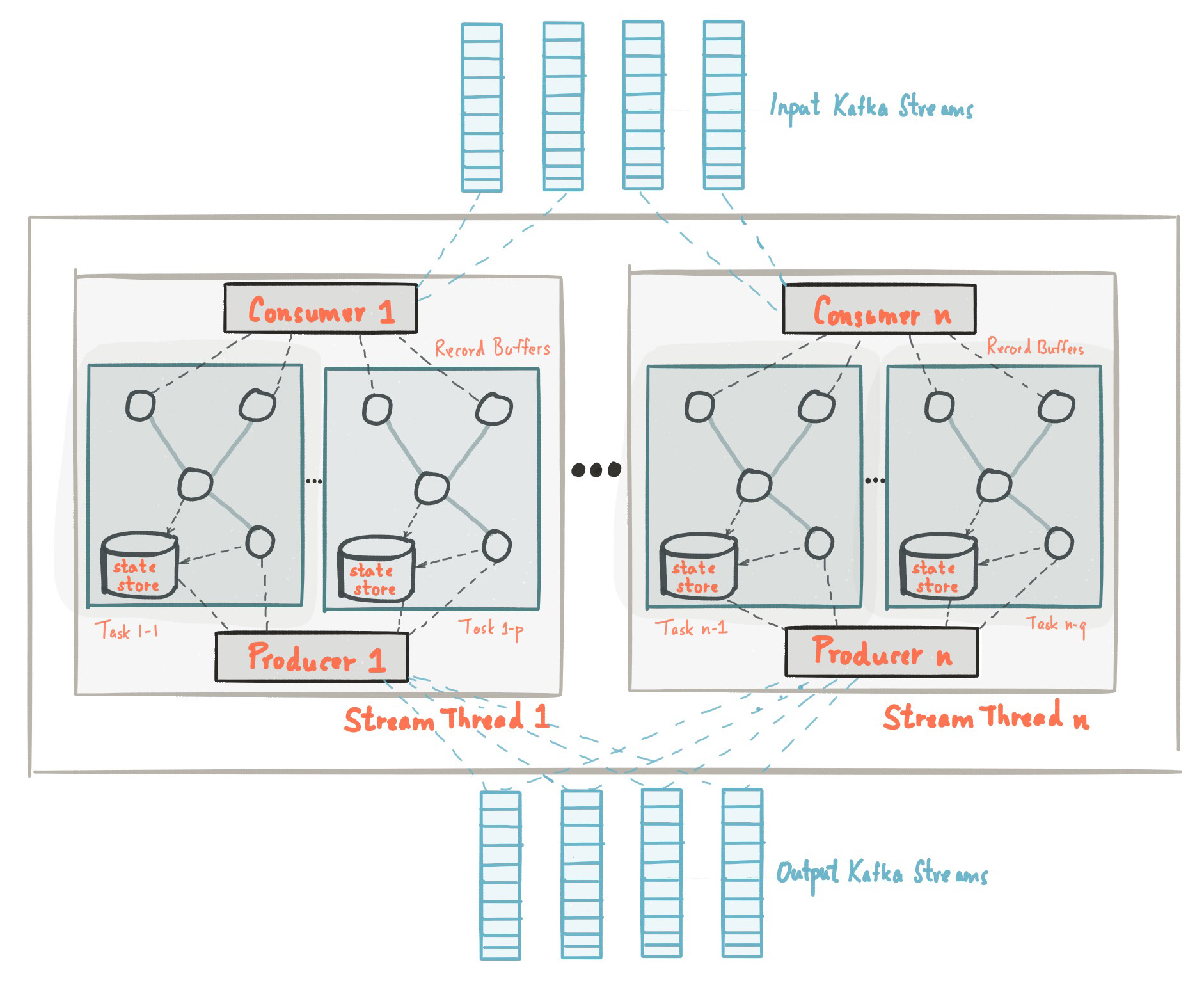
Here is the anatomy of an application that uses the Kafka Streams API. It provides a logical view of a Kafka Streams application that contains multiple stream threads, that each contain multiple stream tasks.
Tip
To learn how Kafka transactions provide you with accurate, repeatable results from chains of many stream processors or microservices, connected via event streams, see Building Systems Using Transactions in Apache Kafka.
Processor topology
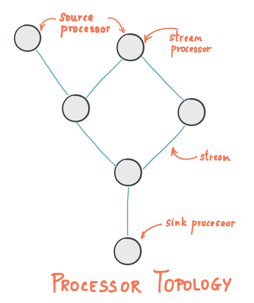
A processor topology or simply topology defines the stream processing computational logic for your application, i.e., how input data is transformed into output data. A topology is a graph of stream processors (nodes) that are connected by streams (edges) or shared state stores. There are two special processors in the topology:
Source Processor: A source processor is a special type of stream processor that does not have any upstream processors. It produces an input stream to its topology from one or multiple Kafka topics by consuming records from these topics and forward them to its down-stream processors.
Sink Processor: A sink processor is a special type of stream processor that does not have down-stream processors. It sends any received records from its up-stream processors to a specified Kafka topic.
A stream processing application – i.e., your application – may define one or more such topologies, though typically it defines only one. Developers can define topologies either via the low-level Processor API or via the Kafka Streams DSL, which builds on top of the former.
A processor topology is merely a logical abstraction for your stream processing code. At runtime, the logical topology is instantiated and replicated inside the application for parallel processing (see Parallelism model).
Parallelism model
Stream partitions and tasks
The messaging layer of Kafka partitions data for storing and transporting it. Kafka Streams partitions data for processing it. In both cases, this partitioning is what enables data locality, elasticity, scalability, high performance, and fault tolerance.
Kafka Streams uses the concepts of stream partitions and stream tasks as logical units of its parallelism model. There are close links between Kafka Streams and Kafka in the context of parallelism:
Each stream partition is a totally ordered sequence of data records and maps to a Kafka topic partition.
A data record in the stream maps to a Kafka message from that topic.
The keys of data records determine the partitioning of data in both Kafka and Kafka Streams, i.e., how data is routed to specific partitions within topics.
An application’s processor topology is scaled by breaking it into multiple stream tasks. More specifically, Kafka Streams creates a fixed number of stream tasks based on the input stream partitions for the application, with each task being assigned a list of partitions from the input streams (i.e., Kafka topics). The assignment of stream partitions to stream tasks never changes, hence the stream task is a fixed unit of parallelism of the application. Tasks can then instantiate their own processor topology based on the assigned partitions; they also maintain a buffer for each of its assigned partitions and process input data one-record-at-a-time from these record buffers. As a result stream tasks can be processed independently and in parallel without manual intervention.
Slightly simplified, the maximum parallelism at which your application may run is bounded by the maximum number of stream tasks, which itself is determined by maximum number of partitions of the input topic(s) the application is reading from. For example, if your input topic has 5 partitions, then you can run up to 5 applications instances. These instances will collaboratively process the topic’s data. If you run a larger number of app instances than partitions of the input topic, the “excess” app instances will launch but remain idle; however, if one of the busy instances goes down, one of the idle instances will resume the former’s work. We provide a more detailed explanation and example in the FAQ.
Sub-topologies (also called sub-graphs)
If there are multiple processor topologies specified in a Kafka Streams application, each task instantiates only one of the topologies for processing. In addition, a single processor topology may be decomposed into independent sub-topologies (or sub-graphs).
A sub-topology is a set of processors, that are all transitively connected as parent/child or via state stores in the topology, so different sub-topologies exchange data via topics and don’t share any state stores. Each task may instantiate only one such sub-topology for processing. This further scales out the computational workload to multiple tasks.
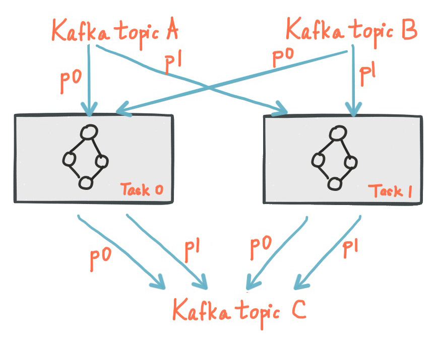
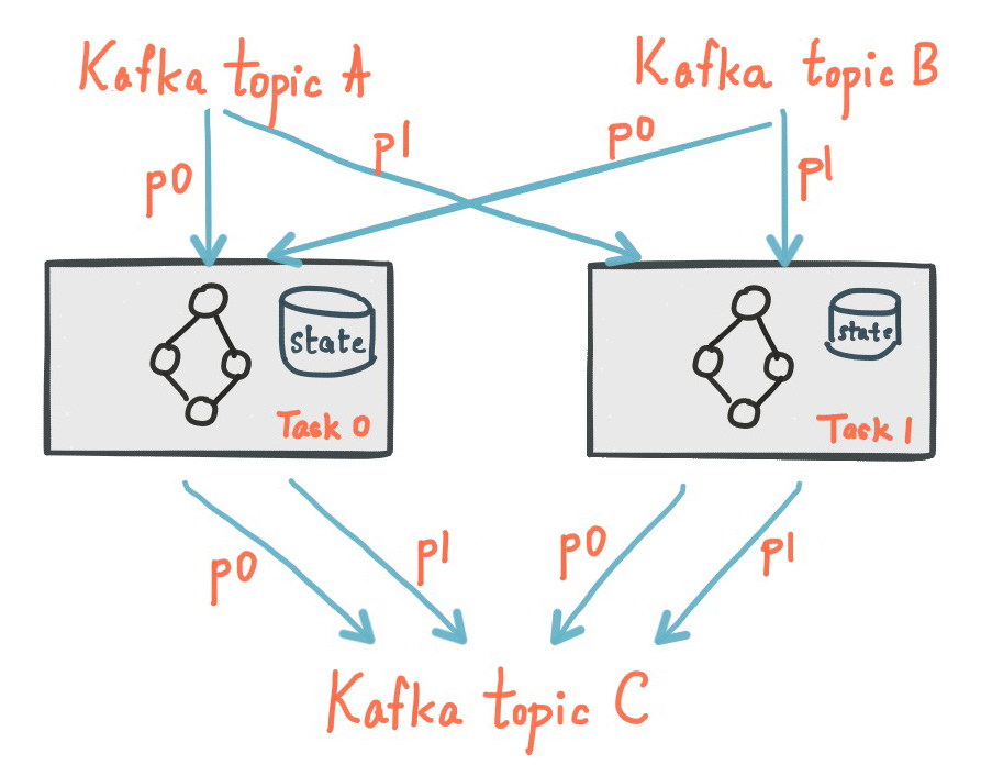
Two tasks each assigned with one partition of the input streams.
It’s important to understand that Kafka Streams is not a resource manager, but a library that “runs” anywhere its stream processing application runs. Multiple instances of the application are executed either on the same machine, or spread across multiple machines and tasks can be distributed automatically by the library to those running application instances. The assignment of partitions to tasks never changes; if an application instance fails, all its assigned tasks will be restarted on other instances and continue to consume from the same stream partitions.
Topic partitions are assigned to tasks, and tasks are assigned to all threads over all instances, in a best-effort attempt to trade off load-balancing and stickiness of stateful tasks. For this assignment, Kafka Streams uses the StreamsPartitionAssignor class and doesn’t let you change to a different assignor. If you try to use a different assignor, Kafka Streams ignores it.
Threading model
Kafka Streams allows the user to configure the number of threads that the library can use to parallelize processing within an application instance. Each thread can execute one or more stream tasks with their processor topologies independently.
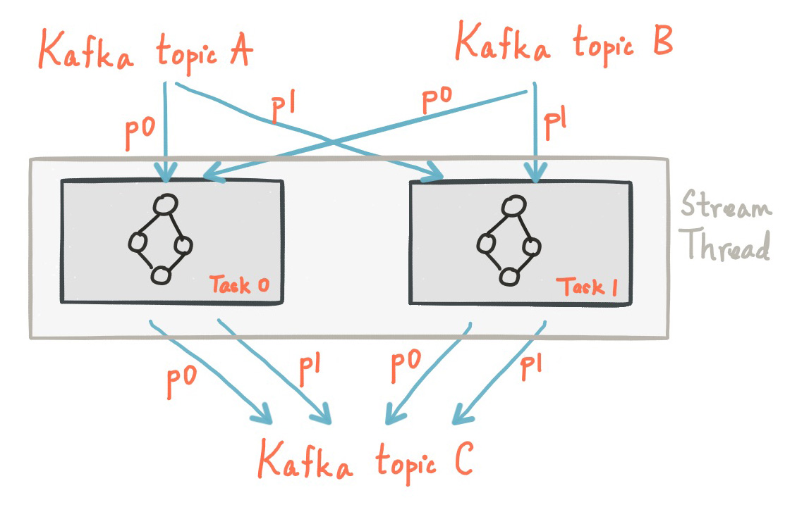
One stream thread running two stream tasks.
Starting more stream threads or more instances of the application merely amounts to replicating the topology and having it process a different subset of Kafka partitions, effectively parallelizing processing. It is worth noting that there is no shared state amongst the threads, so no inter-thread coordination is necessary. This makes it very simple to run topologies in parallel across the application instances and threads. The assignment of Kafka topic partitions amongst the various stream threads is transparently handled by Kafka Streams leveraging Kafka’s server-side coordination functionality.
As we described above, scaling your stream processing application with Kafka Streams is easy: you merely need to start additional instances of your application, and Kafka Streams takes care of distributing partitions across stream tasks that run in the application instances. You can start as many threads of the application as there are input Kafka topic partitions so that, across all running instances of an application, every thread (or rather, the stream tasks that the thread executes) has at least one input partition to process.
As of Kafka 2.8 you can scale stream threads much in the same way that you can scale your Kafka Streams clients. Simply add or remove stream threads and Kafka Streams takes care of redistributing the partitions. You may also add threads to replace stream threads that have died, eliminating the need to restart clients to recover the number of running threads.
Example
To understand the parallelism model that Kafka Streams offers, let’s walk through an example.
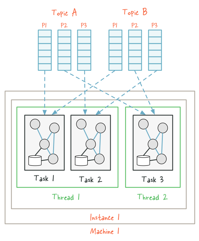
Imagine a Kafka Streams application that consumes from two topics, A and B, with each having 3 partitions. If we now start the application on a single machine with the number of threads configured to 2, we end up with two stream threads instance1-thread1 and instance1-thread2. Kafka Streams will break this topology into three tasks because the maximum number of partitions across the input topics A and B is max(3, 3) == 3, and then distribute the six input topic partitions evenly across these three tasks; in this case, each task will process records from one partition of each input topic, for a total of two input partitions per task. Finally, these three tasks will be spread evenly – to the extent this is possible – across the two available threads, which in this example means that the first thread will run 2 tasks (consuming from 4 partitions) and the second thread will run 1 task (consuming from 2 partitions).
Now imagine we want to scale out this application later on, perhaps because the data volume has increased significantly. We decide to start running the same application but with only a single thread on another, different machine. A new thread instance2-thread1 will be created, and input partitions will be re-assigned similar to:
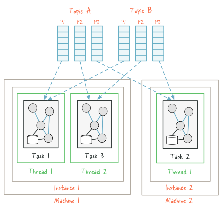
When the re-assignment occurs, some partitions – and hence their corresponding tasks including any local state stores – will be “migrated” from the existing threads to the newly added threads (here, stream task 2 from instance1-thread1 on the first machine was migrated to instance2-thread1 on the second machine). As a result, Kafka Streams has effectively rebalanced the workload among instances of the application at the granularity of Kafka topic partitions.
What if we wanted to add even more instances of the same application? We can do so until a certain point, which is when the number of running instances is equal to the number of available input partitions to read from. At this point, before it would make sense to start further application instances, we would first need to increase the number of partitions for topics A and B; otherwise, we would over-provision the application, ending up with idle instances that are waiting for partitions to be assigned to them, which may never happen.
State
Kafka Streams provides so-called state stores, which can be used by stream processing applications to store and query data, which is an important capability when implementing stateful operations. The Kafka Streams DSL, for example, automatically creates and manages such state stores when you are calling stateful operators such as count() or aggregate(), or when you are windowing a stream.
Every stream task in a Kafka Streams application may embed one or more local state stores that can be accessed via APIs to store and query data required for processing. These state stores can either be a RocksDB database, an in-memory hash map, or another convenient data structure. Kafka Streams offers fault-tolerance and automatic recovery for local state stores.
Two stream tasks with their dedicated local state stores
A Kafka Streams application is typically running on many application instances. Because Kafka Streams partitions the data for processing it, an application’s entire state is spread across the local state stores of the application’s running instances. The Kafka Streams API lets you work with an application’s state stores both locally (e.g., on the level of an instance of the application) as well as in its entirety (on the level of the “logical” application), for example through stateful operations such as count() or through Interactive Queries.
Depth-first processing strategy
Kafka Streams defines its processing logic through a processor topology, which is a graph of stream processors connected by streams. When a record enters this topology, it’s processed by one stream processor, which forwards the transformed record to its downstream processors.
While a strict “depth-first” or “breadth-first” strategy isn’t explicitly defined for the overall processing of all records across all partitions at once, when a single record is processed through its chain of connected processors within a task, the processing generally follows the defined links in the topology. This resembles a depth-first traversal for the specific record’s path through the graph, which means that a record goes as far down a processing path as possible before the task processes another record. Each record consumed from Kafka goes through the whole processor (sub-)topology for processing and for (possibly) being written back to Kafka before the next record is processed. For a given StreamsTask, only one message is processed at a time.
For each task, there is a single state store, so a state store is accessed only from the same sub-topology, which means there is never a read/write race condition when accessing a state store.
Memory management
Record caches
With Kafka Streams, you can specify the total memory (RAM) size that is used for an instance of a processing topology. This memory is used for internal caching and compacting of records before they are written to state stores, or forwarded downstream to other nodes. These caches differ slightly in implementation in the DSL and Processor API.
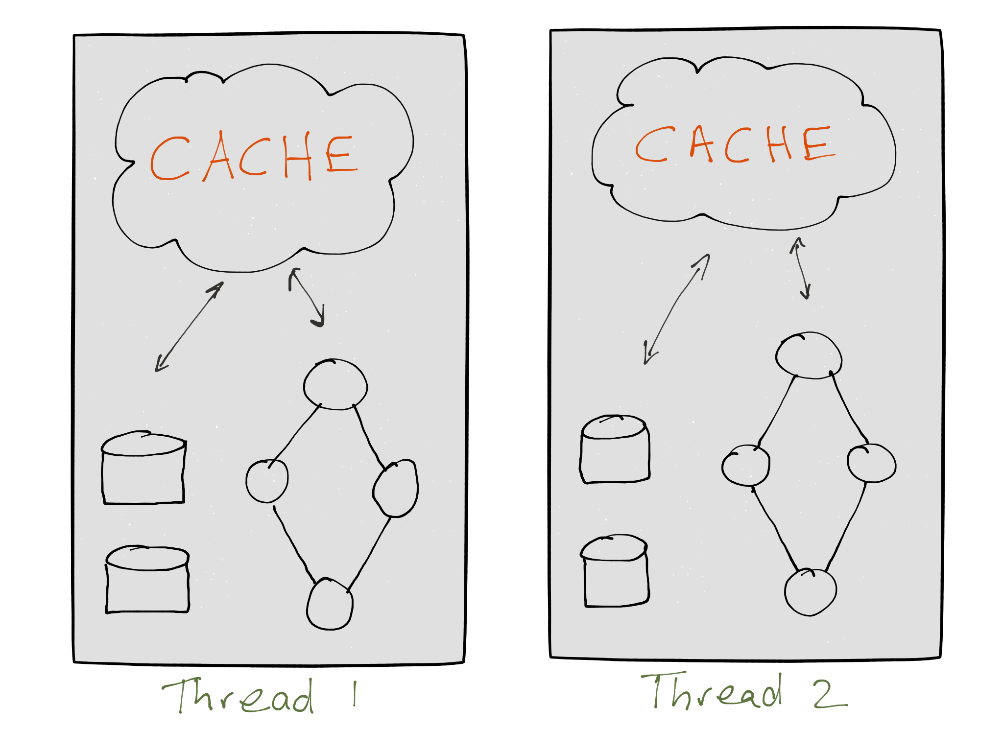
The specified cache size is divided equally among the Kafka Stream threads of a topology. Memory is shared over all threads per instance. Each thread maintains a memory pool accessible by its tasks’ processor nodes for caching. Specifically, this is used by stateful processor nodes that perform aggregates and thus have a state store.
The cache has three functions. First, it serves as a read cache to speed up reading data from a state store. Second, it serves as a write-back buffer for a state store. A write-back cache allows for batching multiple records instead of sending each record individually to the state store. It also reduces the number of requests going to a state store (and its changelog topic stored in Kafka if it is a persistent state store) because records with the same key are compacted in cache. Third, the write-back cache reduces the number of records going to downstream processor nodes as well.
Thus, without requiring you to invoke any explicit processing operators in the API, these caches allow you to make trade-off decisions between:
When using smaller cache sizes: larger rate of downstream updates with shorter intervals between updates.
When using larger cache sizes: smaller rate of downstream updates with larger intervals between updates. Typically, this results reduced network IO to Kafka and reduced local disk IO to RocksDB-backed state stores, for example.
The final computation results are identical regardless of the cache size (including a disabled cache), which means it is safe to enable or disable the cache. It is not possible to predict when or how updates will be compacted because this depends on many factors, including:
Cache size.
Characteristics of the data being processed.
Configuration parameters, for example
commit.interval.ms.
For more information, see Kafka Streams Memory Management for Confluent Platform in the Developer Guide.
Fault tolerance
Kafka Streams builds on fault-tolerance capabilities integrated natively within Kafka. Kafka partitions are highly available and replicated; so when stream data is persisted to Kafka it is available even if the application fails and needs to re-process it. Tasks in Kafka Streams leverage the fault-tolerance capability offered by the Kafka consumer client to handle failures. If a task runs on a machine that fails, Kafka Streams automatically restarts the task in one of the remaining running instances of the application.
In addition, Kafka Streams makes sure that the local state stores are robust to failures, too. For each state store, it maintains a replicated changelog Kafka topic in which it tracks any state updates. These changelog topics are partitioned as well so that each local state store instance, and hence the task accessing the store, has its own dedicated changelog topic partition. Log compaction is enabled on the changelog topics so that old data can be purged safely to prevent the topics from growing indefinitely. If tasks run on a machine that fails and are restarted on another machine, Kafka Streams guarantees to restore their associated state stores to the content before the failure by replaying the corresponding changelog topics prior to resuming the processing on the newly started tasks. As a result, failure handling is completely transparent to the end user.
Tip
Optimization: The cost of task (re)initialization typically depends primarily on the time for restoring the state by replaying the state stores’ associated changelog topics. To minimize this restoration time, you can configure your applications to have standby replicas of local states, which are fully replicated copies of the state. When a task migration happens, Kafka Streams assigns a task to an application instance where such a standby replica already exists, to minimize the task (re)initialization cost. For more information, see num.standby.replicas at Optional configuration parameters in the Developer Guide. Starting in 2.6, Kafka Streams guarantees that a task is assigned to an instance with a fully caught-up local copy of the state exists, if such an instance exists. Standby tasks increase the likelihood that a caught-up instance exists in the case of a failure.
Important
The restore consumer is also used for standby tasks.
You can also configure standby replicas with rack awareness. When configured, Kafka Streams attempts to distribute a standby task on a different “rack” than the active one, thus having a faster recovery time when the rack of the active tasks fails. For more information, see rack.aware.assignment.tags.
There is also a client config named client.rack which can set the rack for a Kafka consumer. If brokers also have their rack set by using broker.rack, then rack-aware task assignment can be enabled via rack.aware.assignment.strategy to compute a task assignment which can reduce cross-rack traffic by trying to assign tasks to clients with the same rack.
You can also use client.rack to distribute standby tasks to different racks from the active ones, which has a similar functionality as rack.aware.assignment.tags. Currently, rack.aware.assignment.tag takes precedence in distributing standby tasks, which means if both configs are present, rack.aware.assignment.tag is used for distributing standby tasks on different racks from the active ones, because it can configure more tag keys.
Local State Consistency
When state is updated, it’s written to a local state store and to an internal changelog topic. Kafka Streams keeps the changelog topic and local state in sync.
Exactly Once Semantics (EOS)
If Exactly Once Semantics (EOS) is enabled and the local state diverges from the changelog topic, Kafka Streams deletes the state store and rebuilds it from the changelog.
If a write to the changelog fails for a retryable reason, Kafka Streams keeps trying to write, but if it fails fatally, it crashes and on restart detects that the state store is “ahead” of the latest offset in the changelog, or it may detect an unclean shutdown, indicating dirty state. Kafka Streams proceeds to rebuild state from the changelog.
Kafka Streams knows what changelog offset is represented in the state store by using a client-local “checkpoint file” that stores metadata only. This checkpoint file is present only when Kafka Streams knows that the state is consistent with the changelog.
When Kafka Streams detects an inconsistency, the entire state store is discarded and rebuilt from the changelog, which can be expensive but occurs rarely. This can occur if Kafka Streams crashes during processing, or if the brokers enter a bad state and are unable to accept writes. A similar process of building the state store from scratch also can happen on rebalance, for example, if a task moves to a node that didn’t previously host it.
At-least-once Semantics (ALOS)
For the non-EOS case, Kafka Streams may have “dirty” writes, and no state rebuild is attempted, because this is what the at-least-once processing guarantees provides.
With non-EOS, Kafka Streams only ensures that the store is flushed to disk, and the changelogs write to Kafka before Kafka Streams commits the corresponding offsets and before it updates the checkpoint file.
If there is an error between two commits, Kafka Streams re-uses the state store and changelog topic as-is. Before data processing resumes, it replays the tail of the changelog, which means that Kafka Streams reads the changelog from the checkpointed offsets to its end. This guarantees that any writes to the changelog topic are also in the store and keeps both in sync.
Flow control with timestamps
Kafka Streams regulates the progress of streams by the timestamps of data records by attempting to synchronize all source streams in terms of time. By default, Kafka Streams will provide your application with event-time processing semantics. This is important especially when an application is processing multiple streams (i.e., Kafka topics) with a large amount of historical data. For example, a user may want to re-process past data in case the business logic of an application was changed significantly, e.g. to fix a bug in an analytics algorithm. Now it is easy to retrieve a large amount of past data from Kafka; however, without proper flow control, the processing of the data across topic partitions may become out-of-sync and produce incorrect results.
As mentioned in the Concepts section, each data record in Kafka Streams is associated with a timestamp. Based on the timestamps of the records in its stream record buffer, stream tasks determine the next assigned partition to process among all its input streams. However, Kafka Streams does not reorder records within a single stream for processing since reordering would break the delivery semantics of Kafka and make it difficult to recover in the face of failure. This flow control is best-effort because it is not always possible to strictly enforce execution order across streams by record timestamp; in fact, in order to enforce strict execution ordering, one must either wait until the system has received all the records from all streams (which may be quite infeasible in practice) or inject additional information about timestamp boundaries or heuristic estimates such as MillWheel’s watermarks.
Backpressure
Kafka Streams does not use a backpressure mechanism because it does not need one. Using a depth-first processing strategy, each record consumed from Kafka will go through the whole processor (sub-)topology for processing and for (possibly) being written back to Kafka before the next record will be processed. As a result, no records are being buffered in-memory between two connected stream processors. Also, Kafka Streams leverages Kafka’s consumer client behind the scenes, which works with a pull-based messaging model that allows downstream processors to control the pace at which incoming data records are being read.
The same applies to the case of a processor topology that contains multiple independent sub-topologies, which will be processed independently from each other (cf. Parallelism model). For example, the following code defines a topology with two independent sub-topologies:
stream1.to("my-topic");
stream2 = builder.stream("my-topic");
Any data exchange between sub-topologies will happen through Kafka, i.e. there is no direct data exchange (in the example above, data would be exchanged through the topic “my-topic”). For this reason there is no need for a backpressure mechanism in this scenario, too.
Note
This website includes content developed at the Apache Software Foundation under the terms of the Apache License v2.