Kafka Streams Basics for Confluent Platform
In this section we summarize the key concepts of Kafka Streams. For more detailed information refer to Kafka Streams Architecture for Confluent Platform and the Kafka Streams Developer Guide for Confluent Platform. You may also be interested in the Kafka Streams 101 course.
Kafka 101
Kafka Streams is, by deliberate design, tightly integrated with Apache Kafka®: many capabilities of Kafka Streams such as its stateful processing features, its fault tolerance, and its processing guarantees are built on top of functionality provided by Apache Kafka®’s storage and messaging layer. It is therefore important to familiarize yourself with the key concepts of Kafka, notably the sections Getting Started and Design. In particular you should understand:
The who’s who: Kafka distinguishes producers, consumers, and brokers. In short, producers publish data to Kafka brokers, and consumers read published data from Kafka brokers. Producers and consumers are totally decoupled, and both run outside the Kafka brokers in the perimeter of a Kafka cluster. A Kafka cluster consists of one or more brokers. An application that uses the Kafka Streams API acts as both a producer and a consumer.
The data: Data is stored in topics. The topic is the most important abstraction provided by Kafka: it is a category or feed name to which data is published by producers. Every topic in Kafka is split into one or more partitions. Kafka partitions data for storing, transporting, and replicating it. Kafka Streams partitions data for processing it. In both cases, this partitioning enables elasticity, scalability, high performance, and fault tolerance.
Parallelism: Partitions of Kafka topics, and especially their number for a given topic, are also the main factor that determines the parallelism of Kafka with regards to reading and writing data. Because of the tight integration with Kafka, the parallelism of an application that uses the Kafka Streams API is primarily depending on Kafka’s parallelism.
Stream
A stream is the most important abstraction provided by Kafka Streams: it represents an unbounded, continuously updating data set, where unbounded means “of unknown or of unlimited size”. Just like a topic in Kafka, a stream in the Kafka Streams API consists of one or more stream partitions.
A stream partition is an, ordered, replayable, and fault-tolerant sequence of immutable data records, where a data record is defined as a key-value pair.
Stream Processing Application
A stream processing application is any program that makes use of the Kafka Streams library. In practice, this means it is probably “your” application. It may define its computational logic through one or more processor topologies.
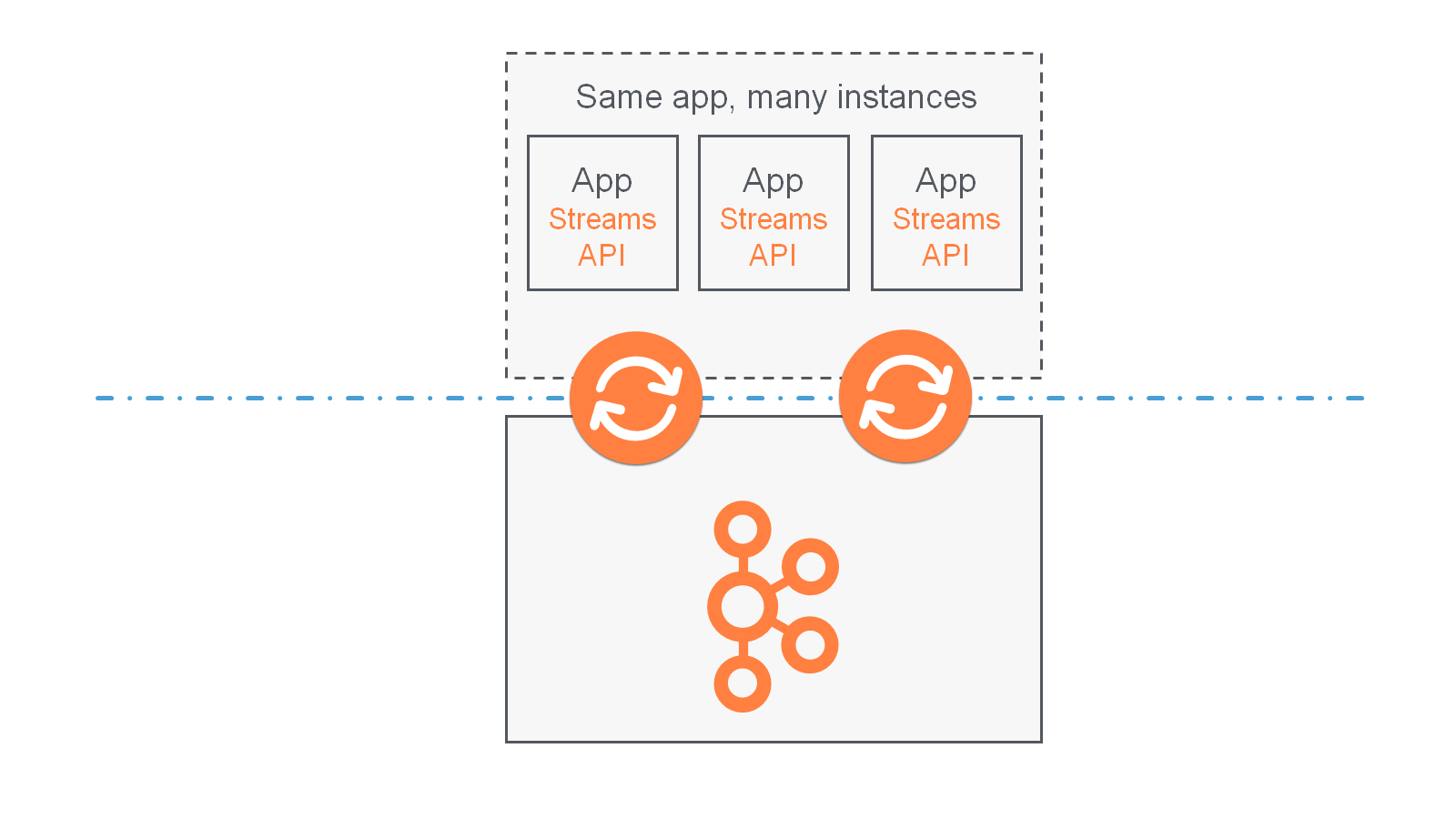
Your stream processing application doesn’t run inside a broker. Instead, it runs in a separate JVM instance, or in a separate cluster entirely.
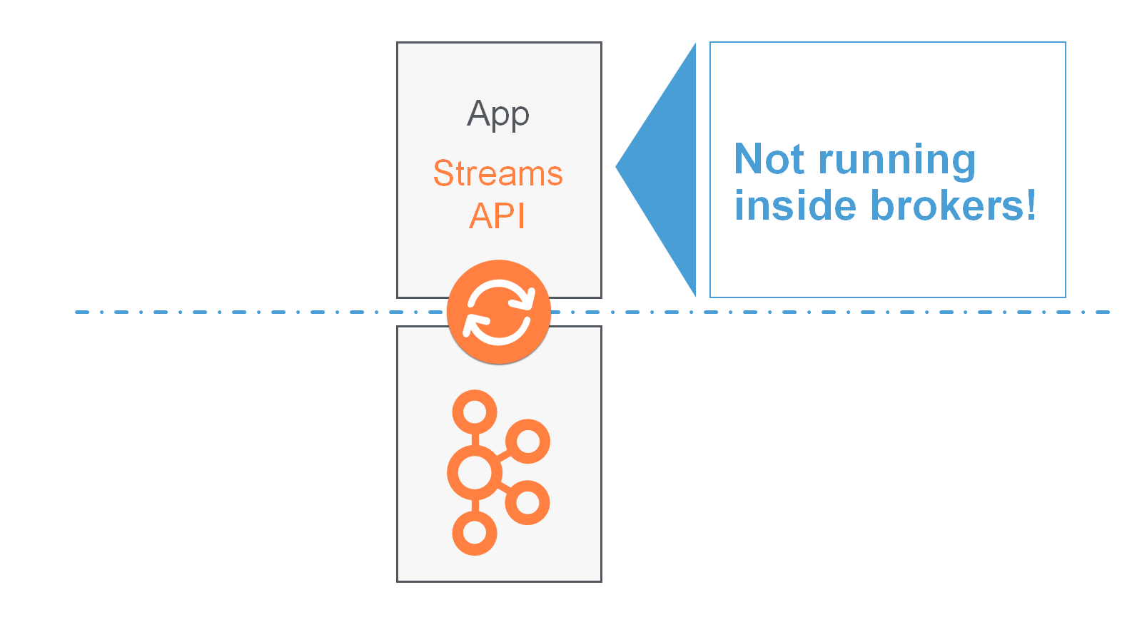
An application instance is any running instance or “copy” of your application. Application instances are the primary means to elasticly scale and parallelize your application, and they also contribute to making it fault-tolerant. For example, you may need the power of ten machines to handle the incoming data load of your application; here, you could opt to run ten instances of your application, one on each machine, and these instances would automatically collaborate on the data processing – even as new instances/machines are added or existing ones removed during live operation.
Processor Topology
A processor topology or simply topology defines the computational logic of the data processing that needs to be performed by a stream processing application. A topology is a graph of stream processors (nodes) that are connected by streams (edges). Developers can define topologies either via the low-level Processor API or via the Kafka Streams DSL, which builds on top of the former.
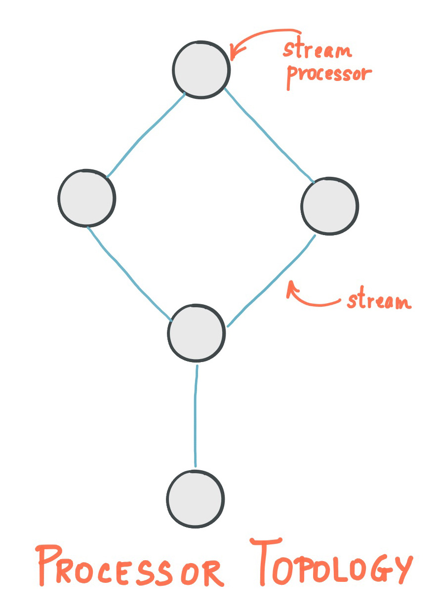
The Architecture documentation describes topologies in more detail.
Stream Processor
A stream processor is a node in the processor topology as shown in the diagram of section Processor Topology. It represents a processing step in a topology, i.e. it is used to transform data. Standard operations such as map or filter, joins, and aggregations are examples of stream processors that are available in Kafka Streams out of the box. A stream processor receives one input record at a time from its upstream processors in the topology, applies its operation to it, and may subsequently produce one or more output records to its downstream processors.
Kafka Streams provides two APIs to define stream processors:
The declarative, functional DSL is the recommended API for most users – and notably for starters – because most data processing use cases can be expressed in just a few lines of DSL code. Here, you typically use built-in operations such as
mapandfilter.The imperative, lower-level Processor API provides you with even more flexibility than the DSL but at the expense of requiring more manual coding work. Here, you can define and connect custom processors as well as directly interact with state stores.
Stateful Stream Processing
Some stream processing applications don’t require state – they are stateless – which means the processing of a message is independent from the processing of other messages. Examples are when you only need to transform one message at a time, or filter out messages based on some condition.
In practice, however, most applications require state – they are stateful – in order to work correctly, and this state must be managed in a fault-tolerant manner. Your application is stateful whenever, for example, it needs to join, aggregate, or window its input data. Kafka Streams provides your application with powerful, elastic, highly scalable, and fault-tolerant stateful processing capabilities.
Duality of Streams and Tables
When implementing stream processing use cases in practice, you typically need both streams and also databases. An example use case that is very common in practice is an e-commerce application that enriches an incoming stream of customer transactions with the latest customer information from a database table. In other words, streams are everywhere, but databases are everywhere, too.
Any stream processing technology must therefore provide first-class support for streams and tables. Kafka’s Streams API provides such functionality through its core abstractions for streams and tables, which we will talk about in a minute. Now, an interesting observation is that there is actually a close relationship between streams and tables, the so-called stream-table duality. And Kafka exploits this duality in many ways: for example, to make your applications elastic, to support fault-tolerant stateful processing, or to run Kafka Streams Interactive Queries for Confluent Platform against your application’s latest processing results. And, beyond its internal usage, the Kafka Streams API also allows developers to exploit this duality in their own applications.
Before we discuss concepts such as aggregations in Kafka Streams we must first introduce tables in more detail, and talk about the aforementioned stream-table duality. Essentially, this duality means that a stream can be viewed as a table, and a table can be viewed as a stream.
The following explanations are kept simple intentionally and skip the discussion of compound keys, multisets, and so on.
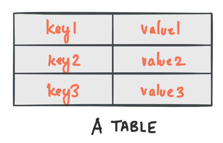
A simple form of a table is a collection of key-value pairs, also called a map or associative array. Such a table may look as follows:
The stream-table duality describes the close relationship between streams and tables.
Stream as Table: A stream can be considered a changelog of a table, where each data record in the stream captures a state change of the table. A stream is thus a table in disguise, and it can be easily turned into a “real” table by replaying the changelog from beginning to end to reconstruct the table. Similarly, aggregating data records in a stream will return a table. For example, we could compute the total number of pageviews by user from an input stream of pageview events, and the result would be a table, with the table key being the user and the value being the corresponding pageview count.
Table as Stream: A table can be considered a snapshot, at a point in time, of the latest value for each key in a stream (a stream’s data records are key-value pairs). A table is thus a stream in disguise, and it can be easily turned into a “real” stream by iterating over each key-value entry in the table.
Let’s illustrate this with an example. Imagine a table that tracks the total number of pageviews by user (first column of diagram below). Over time, whenever a new pageview event is processed, the state of the table is updated accordingly. Here, the state changes between different points in time – and different revisions of the table – can be represented as a changelog stream (second column).
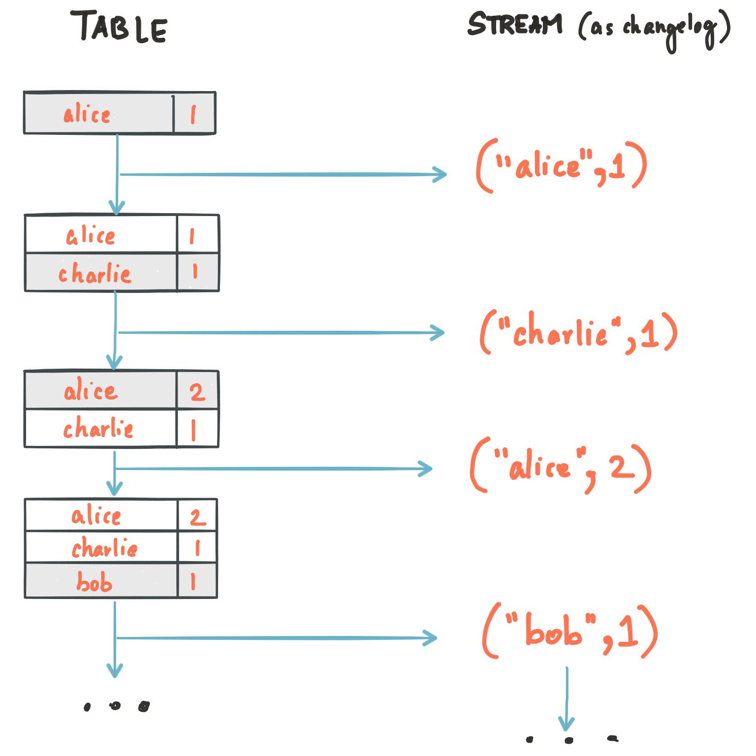
Because of the stream-table duality, the same stream can be used to reconstruct the original table (third column):
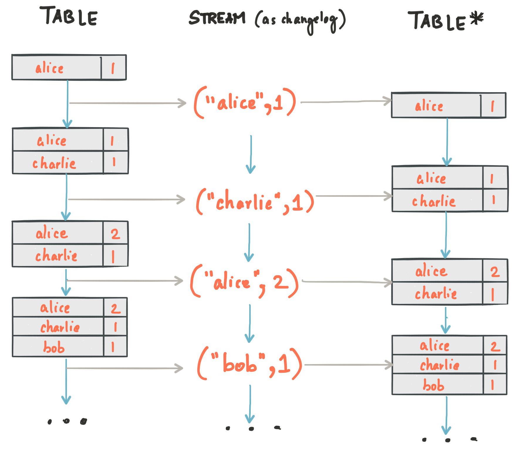
The same mechanism is used, for example, to replicate databases via change data capture (CDC) and, within Kafka Streams, to replicate its so-called state stores across machines for fault tolerance. The stream-table duality is such an important concept for stream processing applications in practice that Kafka Streams models it explicitly via the KStream and KTable abstractions, which we describe in the next sections.
KStream
A KStream is an abstraction of a record stream, where each data record represents a self-contained datum in the unbounded data set. Using the table analogy, data records in a record stream are always interpreted as an “INSERT” – think: adding more entries to an append-only ledger – because no record replaces an existing row with the same key. Examples are a credit card transaction, a page view event, or a server log entry.
Only the Kafka Streams DSL has the notion of a KStream.
To illustrate, imagine the following two data records are being sent to the stream:
("alice", 1) --> ("alice", 3)
If your stream processing application were to sum the values per user, it would return 4 for alice. Why? Because the second data record would not be considered an update of the previous record. Compare this behavior of KStream to KTable below, which would return 3 for alice.
KTable
A KTable is an abstraction of a changelog stream, where each data record represents an update. More precisely, the value in a data record is interpreted as an “UPDATE” of the last value for the same record key, if any (if a corresponding key doesn’t exist yet, the update will be considered an INSERT). Using the table analogy, a data record in a changelog stream is interpreted as an UPSERT aka INSERT/UPDATE because any existing row with the same key is overwritten. Also, null values are interpreted in a special way: a record with a null value represents a “DELETE” or tombstone for the record’s key.
Only the Kafka Streams DSL has the notion of a KTable.
To illustrate, let’s imagine the following two data records are being sent to the stream:
("alice", 1) --> ("alice", 3)
If your stream processing application were to sum the values per user, it would return 3 for alice. Why? Because the second data record would be considered an update of the previous record. Compare this behavior of KTable with the illustration for KStream above, which would return 4 for alice.
You have already seen an example of a changelog stream in the section Duality of Streams and Tables. Another example are change data capture (CDC) records in the changelog of a relational database, representing which row in a database table was inserted, updated, or deleted.
KTable also provides an ability to look up current values of data records by keys. This table-lookup functionality is available through join operations (see also Joining in the Developer Guide) as well as through Interactive Queries.
For more information, see Kafka Streams 101 - KTable.
Effect of Kafka log compaction
Another way of thinking about KStream and KTable is as follows: If you were to store a KTable into a Kafka topic, you’d probably want to enable Kafka’s log compaction feature to save storage space.
But it wouldn’t be safe to enable log compaction in the case of a KStream, because as soon as log compaction begins purging older data records of the same key, it would break the semantics of the data. To pick up the illustration example again, you’d suddenly get a 3 for alice, instead of a 4, because log compaction would have removed the ("alice", 1) data record. this means that log compaction is safe for a KTable (changelog stream) but it is a mistake for a KStream (record stream).
GlobalKTable
Like a KTable, a GlobalKTable is an abstraction of a changelog stream, where each data record represents an update.
Only the Kafka Streams DSL has the notion of a GlobalKTable.
A GlobalKTable differs from a KTable in the data that they are being populated with, i.e. which data from the underlying Kafka topic is being read into the respective table. Slightly simplified, imagine you have an input topic with 5 partitions. In your application, you want to read this topic into a table. Also, you want to run your application across 5 application instances for maximum parallelism.
If you read the input topic into a KTable, then the “local” KTable instance of each application instance will be populated with data from only 1 partition of the topic’s 5 partitions.
If you read the input topic into a GlobalKTable, then the local GlobalKTable instance of each application instance will be populated with data from all partitions of the topic.
GlobalKTable provides the ability to look up current values of data records by keys. This table-lookup functionality is available through join operations (as described in Joining in the Developer Guide) and Kafka Streams Interactive Queries for Confluent Platform.
Benefits of global tables:
You can use global tables to “broadcast” information to all running instances of your application.
Global tables enable more convenient and efficient joins.
Global tables enable star joins.
Global tables are more efficient when chaining multiple joins.
When joining against a global table, the input data doesn’t need to be co-partitioned.
Global tables support “foreign-key” lookups, which means that you can look up data in the table not just by record key, but also by data in the record values. In this case, the join always uses the table’s primary key, and the “foreign key” refers to the stream records. Unlike a stream-table join that always calculates the join based on the stream-record key, a stream-globalKTable join enables you to extract the join key directly from the stream record’s value.
Drawbacks of global tables include:
Increased local storage consumption compared to the (partitioned) KTable, because the entire topic is tracked.
Increased network and Kafka broker load compared to the (partitioned) KTable, because the entire topic is read.
Time
A critical aspect in stream processing is the notion of time, and how it is modeled and integrated. For example, some operations such as Windowing are defined based on time boundaries.
Kafka Streams supports the following notions of time:
event-time
The point in time when an event or data record occurred (that is, was originally created by the source). Achieving event-time semantics typically requires embedding timestamps in the data records at the time a data record is being produced.
Example: If the event is a geo-location change reported by a GPS sensor in a car, then the associated event-time would be the time when the GPS sensor captured the location change.
processing-time
The point in time when the event or data record happens to be processed by the stream processing application (that is, when the record is being consumed). The processing-time may be milliseconds, hours, days, etc. later than the original event-time.
Example: Imagine an analytics application that reads and processes the geo-location data reported from car sensors to present it to a fleet management dashboard. Here, processing-time in the analytics application might be milliseconds or seconds (such as for real-time pipelines based on Kafka and Kafka Streams) or hours (such as for batch pipelines based on Apache Hadoop or Apache Spark) after event-time.
ingestion-time
The point in time when an event or data record is stored in a topic partition by a Kafka broker. Ingestion-time is similar to event-time, as a timestamp gets embedded in the data record itself. The difference is that the timestamp is generated when the record is appended to the target topic by the Kafka broker, not when the record is created at the source. Ingestion-time may approximate event-time reasonably well if we assume that the time difference between creation of the record and its ingestion into Kafka is sufficiently small, where “sufficiently” depends on the specific use case. Thus, ingestion-time may be a reasonable alternative for use cases where event-time semantics are not possible, perhaps because the data producers don’t embed timestamps (such as with older versions of Kafka’s Java producer client) or the producer cannot assign timestamps directly (for example, does not have access to a local clock).
stream-time
The maximum timestamp seen over all processed records so far. Kafka Streams tracks stream-time on a per-task basis.
Timestamps
Kafka Streams assigns a timestamp to every data record via so-called timestamp extractors. These per-record timestamps describe the progress of a stream with regards to time (although records may be out-of-order within the stream) and are leveraged by time-dependent operations such as joins. We call it the event-time of the application to differentiate with the wall-clock-time when this application is actually executing. Event-time is also used to synchronize multiple input streams within the same application.
Concrete implementations of timestamp extractors may retrieve or compute timestamps based on the actual contents of data records such as an embedded timestamp field to provide event-time or ingestion-time semantics, or use any other approach such as returning the current wall-clock time at the time of processing, thereby yielding processing-time semantics to stream processing applications. Developers can thus enforce different notions/semantics of time depending on their business needs.
Finally, whenever a Kafka Streams application writes records to Kafka, then it will also assign timestamps to these new records. The way the timestamps are assigned depends on the context:
When new output records are generated via directly processing some input record, output record timestamps are inherited from input record timestamps directly.
When new output records are generated via periodic functions, the output record timestamp is defined as the current internal time of the stream task.
For aggregations, the timestamp of the resulting update record will be that of the latest input record that triggered the update.
For aggregations and joins, timestamps are computed using the following rules.
For joins (stream-stream, table-table) that have left and right input records, the timestamp of the output record is assigned
max(left.ts, right.ts).For stream-table joins, the output record is assigned the timestamp from the stream record.
For aggregations, Kafka Streams also computes the
maxtimestamp across all records, per key, either globally (for non-windowed) or per-window.Stateless operations are assigned the timestamp of the input record. For
flatMapand siblings that emit multiple records, all output records inherit the timestamp from the corresponding input record.
Assign timestamps to output records with the Processor API
You can change the default behavior in the Processor API by assigning timestamps to output records explicitly when calling #forward().
The forward() method takes two parameters: a key-value pair and a timestamp. The optional timestamp parameter can be used to set the timestamp of the output record explicitly.
The following example shows the explicit assignment of timestamps to output records using the forward() method.
public class MyProcessor implements Processor<String, String> {
  private ProcessorContext context;

  @Override
  public void init(ProcessorContext context) {
    this.context = context;
  }

  @Override
  public void process(String key, String value) {
    // Extract the timestamp from the input record.
    long inputTimestamp = context.timestamp();

    // Process the input record.
    String outputValue = processRecord(value);

    // Assign the timestamp to the output record explicitly.
    // You implement the computeOutputTimestamp method for your use case.
    long outputTimestamp = computeOutputTimestamp(inputTimestamp);
    KeyValue<String, String> outputRecord = KeyValue.pair(key, outputValue);
    context.forward(outputRecord, outputTimestamp);
  }

  @Override
  public void close() {}
}
In this example, the timestamp is extracted from the input record by using the context.timestamp() method. The computeOutputTimestamp() custom method, which you implement, computes the timestamp for the output record. Finally, a new key-value pair is created for the output record by using KeyValue.pair() and calling context.forward() with this pair and the computed timestamp.
Assign timestamps to output records with the Kafka Streams API
You can assign timestamps to output records explicitly in Kafka Streams by using the TimestampExtractor interface. Implement this interface to extract a timestamp from each record and use it for processing-time or event-time semantics.
The following example shows the explicit assignment of timestamps to output records using the TimestampExtractor interface.
public class CustomTimestampExtractor implements TimestampExtractor {
    @Override
    public long extract(ConsumerRecord<Object, Object> record, long previousTimestamp) {
        // Extract timestamp from record
        long timestamp = ...;
        return timestamp;
    }
}

// Use the custom timestamp extractor
KStream<String, String> stream = builder.stream("input-topic", Consumed.with(Serdes.String(), Serdes.String())
        .withTimestampExtractor(new CustomTimestampExtractor()));

// Process records with timestamps
stream.map((key, value) -> new KeyValue<>(key, value.toUpperCase()))
        .to("output-topic", Produced.with(Serdes.String(), Serdes.String()));
In this example, a custom TimestampExtractor extracts a timestamp from each record and returns it as a long value. The custom extractor is used when creating a KStream by calling the withTimestampExtractor() method on the Consumed object.
Once you have a stream with timestamps, you can process records with processing-time or event-time semantics by using methods like windowedBy() or groupByKey().
Other aspects of time
Tip
Know your time: When working with time you should also make sure that additional aspects of time such as time zones and calendars are correctly synchronized – or at least understood and traced – throughout your stream data pipelines. It often helps, for example, to agree on specifying time information in UTC or in Unix time (such as seconds since the epoch). You should also not mix topics with different time semantics.
Aggregations
An aggregation operation takes one input stream or table, and yields a new table by combining multiple input records into a single output record. Examples of aggregations are computing counts or sum.
In the Kafka Streams DSL, an input stream of an aggregation operation can be a KStream or a KTable, but the output stream will always be a KTable. This allows Kafka Streams to update an aggregate value upon the out-of-order arrival of further records after the value was produced and emitted. When such out-of-order arrival happens, the aggregating KStream or KTable emits a new aggregate value. Because the output is a KTable, the new value is considered to overwrite the old value with the same key in subsequent processing steps. For more information on out-of-order records, see Out-of-Order Handling.
See also Kafka Streams 101 - Stateful Operations.
Joins
A join operation merges two input streams and/or tables based on the keys of their data records, and yields a new stream/table.
The join operations available in the Kafka Streams DSL differ based on which kinds of streams and tables are being joined; for example, KStream-KStream joins versus KStream-KTable joins.
See also Kafka Streams 101 - Joins.
Windowing
Windowing lets you control how to group records that have the same key for stateful operations such as aggregations or joins into so-called windows. Windows are tracked per record key.
Windowing operations are available in the Kafka Streams DSL. When working with windows, you can specify a grace period for the window that indicates when window results are final. This grace period controls how long Kafka Streams will wait for out-of-order data records for a window. If a record arrives after the grace period of a window has passed (i.e., record.ts > window-end-time + grace-period), the record is discarded and will not be processed in that window.
Out-of-order records are always possible in the real world and your applications must account for them properly. The system’s time semantics determine how out-of-order records are handled. For processing-time, the semantics are “when the record is being processed”, which means that the notion of out-of-order records is not applicable. Similarly, for ingestion-time, the broker assigns timestamps in ascending order based on topic append order; the timestamp indicates ingestion-time only. Out-of-order records can only be considered for event-time semantics, where timestamps are set by producers specifically to indicate event-time. If two producers write to the same topic partition, there is no guarantee on the event append order.
Kafka Streams is able to properly handle out-of-order records for the relevant time semantics (event-time).
Tip
grace period vs. retention time
The grace period supersedes retention time as a more specific means of defining the amount of time a window should allow for out-of-order events after the window ends. Grace period relates directly to usage of final results for a window and is also a lower bound on retention time.
Retention time is still configurable, but as a lower-level property of the window store. You might choose to retain events for a long time (the default is one day) to support, for example, Interactive Queries even over final windows or even indefinitely on remote, distributed systems with large storage capacity. On the other hand, you might retain events for a short time for an in-memory implementation.
See also Kafka Streams 101 - Windowing.
Interactive Queries
Interactive Queries allow you to treat the stream processing layer as a lightweight embedded database, and to directly query the latest state of your stream processing application. You can do this without having to first materialize that state to external databases or external storage.
Interactive Queries simplify the architecture and lead to more application-centric architectures.
The following diagram juxtapose two architectures: the first does not use Interactive Queries whereas the second architecture does. It depends on the concrete use case to determine which of these architectures is a better fit – the important takeaway is that Kafka Streams and Interactive Queries give you the flexibility to pick and to compose the right one, rather than limiting you to just a single way.
See also Kafka Streams 101 - Interactive Queries.
Tip
Best of both worlds: Of course you also have the option to run hybrid architectures where, for example, your application may be queried interactively but at the same time also shares some of its results with external systems (e.g. via Kafka Connect).
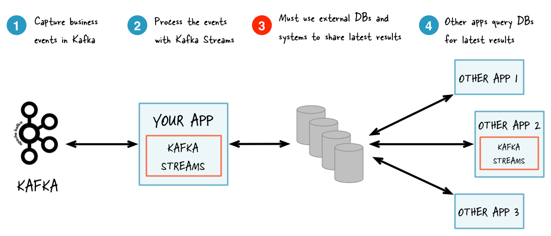
Without Interactive Queries: increased complexity and heavier footprint of architecture.
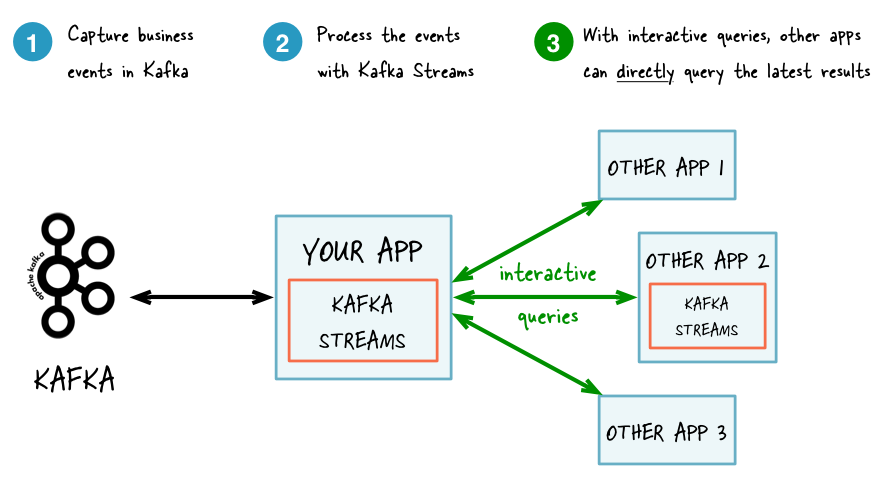
With Interactive Queries: simplified, more application-centric architecture.
Here are some use case examples for applications that benefit from Interactive Queries:
Real-time monitoring: A front-end dashboard that provides threat intelligence (e.g., web servers currently under attack by cyber criminals) can directly query a Kafka Streams application that continuously generates the relevant information by processing network telemetry data in real-time.
Video gaming: A Kafka Streams application continuously tracks location updates from players in the gaming universe. A mobile companion app can then directly query the Kafka Streams application to show the current location of a player to friends and family, and invite them to come along. Similarly, the game vendor can use the data to identify unusual hotspots of players, which may indicate a bug or an operational issue.
Risk and fraud: A Kafka Streams application continuously analyzes user transactions for anomalies and suspicious behavior. An online banking application can directly query the Kafka Streams application when a user logs in to deny access to those users that have been flagged as suspicious.
Trend detection: A Kafka Streams application continuously computes the latest top charts across music genres based on user listening behavior that is collected in real-time. Mobile or desktop applications of a music store can then interactively query for the latest charts while users are browsing the store.
For more information, see the Developer Guide.
Processing Guarantees
Kafka Streams supports at-least-once and exactly-once processing guarantees.
- At-least-once semantics
Records are never lost but may be redelivered. If your stream processing application fails, no data records are lost and fail to be processed, but some data records may be re-read and therefore re-processed. At-least-once semantics is enabled by default (
processing.guarantee="at_least_once") in your Streams configuration.- Exactly-once semantics
Records are processed once. Even if a producer sends a duplicate record, it is written to the broker exactly once. Exactly-once stream processing is the ability to execute a read-process-write operation exactly one time. All of the processing happens exactly once, including the processing and the materialized state created by the processing job that is written back to Kafka. To enable exactly-once semantics, set
processing.guarantee="exactly_once_v2"in your Streams configuration.
When publishing a record with exactly-once semantics enabled, a write is not considered successful until it is acknowledged, and a commit is made to “finalize” the write. After a published record is acknowledged, it cannot be lost as long as a broker that replicates the partition that the record is written to remains “alive”. If a producer attempts to publish a record and experiences a network error, it cannot determine whether this error happened before or after the record was acknowledged. If a producer fails to receive a response that a record was acknowledged, it will resend the record.
Using exactly-once, producers are configured for idempotent writes. This ensures that a retry on a send record does not result in duplicates, and each record is written to the log exactly once. With exactly-once, multiple records are grouped into a single transaction, and so either all or none of the records are committed.
All Kafka replicas have the same log with the same offsets and the consumer controls its position in this log. But if the consumer fails, and the topic partition needs to be taken over by another process, the new process must choose an appropriate starting position.
When the consumer reads records, it processes the records and saves its position. There is a possibility that the consumer process crashes after processing records but before saving its position. In this case, when the new process takes over, the first few records it receives have already been processed. This corresponds to the “at-least-once” semantics in the case of consumer failure.
The consumer’s position is stored as a record in a topic. Using exactly-once semantics, a single transaction writes the offset and sends the processed data to the output topics. If the transaction is aborted, the consumer’s position reverts to its previous value, and the produced data on the output topics are not visible to other consumers, depending on their “isolation level.”
In the default “read_uncommitted” isolation level, all records are visible to consumers, even if they were part of an aborted transaction. In the “read_committed” isolation level, the consumer returns only records from transactions that were committed and any records that were not part of a transaction.
Enforce EOS for Kafka Streams when performing stateful operations
When you perform stateful operations with the at-least-once processing guarantee, a message is persisted into the state store, produced into the output topic, and committed. These operations are triggered sequentially, but their executions are independent and asynchronous.
Consider the cases in which the message is persisted into the state store but the message fails to be produced to the output topic, or the message is produced but fails to be committed. The message is reprocessed, but the result might be inconsistent, generating either a duplicate record or a data loss.
For example, a deduplication app may store the first occurrence of a message but fail to produce to the output topic. It reprocesses the same message, but because it has been stored already in the state store, the reprocessed message is considered a duplicate, is skipped, and isn’t produced to the output topic.
To handle this kind of subtle error, consider using the exactly-once processing guarantee, so the state-store persistence, data production, and commit are coupled in the same transaction, guaranteeing state consistency when reprocessing.
For more information, see the blog post Exactly-once Semantics are Possible: Here’s How Kafka Does it.
Out-of-Order Handling
Beside the guarantee that each record will be processed exactly-once, another challenging issue that many stream processing applications face is how to handle out-of-order data that may impact their business logic. In Kafka Streams, there are two causes that could potentially result in out-of-order data arrivals with respect to their timestamps:
Within a topic partition, a record’s timestamp may not be monotonically increasing along with their offsets. Because Kafka Streams always tries to process records following the offset order, it can cause records with larger timestamps (but smaller offsets) to be processed earlier than records with smaller timestamps (but larger offsets) in the same topic-partition.
A stream task may be processing multiple topic partitions, and if the application is configured not to wait for all partitions to contain some buffered data and to pick from the partition with the smallest timestamp to process the next record, records fetched later for other topic partitions may have timestamps that are smaller than the processed records, effectively causing older records to be processed after the newer records. For more information, see max.task.idle.ms.
For stateless operations, out-of-order data doesn’t impact processing logic, because only one record is considered at a time, without looking into the history of past processed records.
For stateful operations, like aggregations and joins, out-of-order data can cause your processing logic to be incorrect. If you need to handle such out-of-order data, generally you need to allow your applications to wait for a longer time while bookkeeping their states during the wait time, which means making trade-off decisions between latency, cost, and correctness. In Kafka Streams, you can configure your window operators for windowed aggregations to achieve such trade-offs. For more information, see the Developer Guide.
Out-of-Order Terminology
The term order can refer to either offset order or timestamp order. Kafka brokers guarantee offset order, which means that all consumers read all messages in the same order per partition. But Kafka doesn’t provide any guarantee about timestamp order, so records in a topic aren’t ordered by their timestamp and can be “out-of-order” and not monotonically increasing. Because Kafka requires that records are consumed in offset order, Kafka Streams inherits this pattern, so from the perspective of timestamps, Kafka Streams may process records “out-of-order”.
To enable consistent usage and understanding of ordering concepts, use the following definitions.
order: If not explicitly specified, “order” means “timestamp order” in the context of Kafka Streams. This differs from a plain broker/client context, where “order” means “offset order”.
out-of-order: Records that don’t increase monotonically in stream time. For windowed operations, handling out-of-order data requires a grace period.
late: Records that arrive after a window is closed, which means that they arrive after the window-end timestamp plus the grace-period. These records are dropped and not processed. Dropping late records applies only to the corresponding window operator, and the record still may be processed by other operators. You can measure the average and maximum lateness for a task by using the record-lateness-* metrics.
Suggested Reading
Streams and Tables in Apache Kafka: Topics, Partitions, and Storage Fundamentals
Streams and Tables in Apache Kafka: Processing Fundamentals with Kafka Streams and ksqlDB
Streams and Tables in Apache Kafka: Elasticity, Fault Tolerance, and Other Advanced Concepts
Note
This website includes content developed at the Apache Software Foundation under the terms of the Apache License v2.